Geoprocessing with GRASS

During the workshop, we aim to introduce you to the basic concepts of geospatial processing and modeling with GRASS GIS.

Instructor

Dr. Corey T. White is a geospatial scientist and educator with over 20 years of experience in the field of geospatial science. He is the founder of OpenPlains, an interactive geospatial modeling platform for climate-resilience. Dr. White has a Ph.D. in Geospatial Analytics from North Carolina State University and teaches geospatial modeling and UAS mapping at the Center for Geospatial Analytics at NC State University.

Workshop Objective

At the end of this workshop, you will be able to:

Understand the basic concepts of GIS
Understand the basic concepts of geoprocessing
Understand the fundamentals of GRASS GIS
Perform basic geoprocessing tasks with GRASS GIS
Understand how to use GRASS GIS in a Jupyter notebook
Develop a basic workflow for geoprocessing tasks
Publish a basic web map with geoprocessing results

Install GRASS GIS and Data in Google Colab

Google Colab is a free cloud service that allows you to run Python code in a Jupyter notebook environment. We will use Google Colab to run GRASS GIS and perform geoprocessing tasks.

%%bash

apt-get install grass grass-dev grass-doc
# leave the directory with source code
cd ~

# download sample data
mkdir -p grassdata
mkdir -p output
curl -SL https://grass.osgeo.org/sampledata/north_carolina/nc_basic_spm_grass7.zip > nc_basic_spm_grass7.zip
unzip -qq nc_basic_spm_grass7.zip
mv nc_basic_spm_grass7 grassdata
rm nc_basic_spm_grass7.zip

curl -SL https://storage.googleapis.com/public_grassdata/ncssm_workshop_data/ncssm.zip > ncssm.zip
unzip -qq ncssm.zip
mv ncssm grassdata/nc_basic_spm_grass7
rm ncssm.zip

Change the directory in Goolge to the user directory.

import os
os.chdir(os.path.expanduser("~"))

What is GIS?

GIS (Geographic Information System) is a system designed to capture, store, manipulate, analyze, manage, and present spatial or geographic data. GIS applications are tools that allow users to create interactive queries (user-created searches), analyze spatial information, edit data in maps, and present the results of all these operations.

Geospatial data

Geospatial data is data that is associated with a particular location on the surface of the Earth. This data can be represented in many forms, such as vector data (points, lines, polygons), and raster data. Geospatial data can be used to answer questions such as “Where is the nearest hospital?” or “What is the likelihood of flooding at a given location?”.

Raster Data

Raster are a way of represent continuous or discrete spatial data in a grid format. Each cell in the grid has a value that represents a particular attribute. For example, a raster could represent the temperature of the Earth’s surface, with each cell representing the temperature at a particular location.

Vector Data

Vector data is represented as points, lines, and polygons on a map. Points are used to represent specific locations, such as the location of a tree or a building. Lines are used to represent linear features, such as roads or rivers. Polygons are used to represent areas, such as the boundaries of a city or a forest.

Geospatial Data Collection

Geospatial data is collected in many ways, such as:

Earth Observation Systems (Satellites, Aircraft, UAS)

System	Spatial Resolution	Temporal Resolution
UAS	2cm to 5cm RGB, Variable	Multiple times daily
PlanetScope	3m RGB-NIR	Daily
Landsat 8	30m multispectral, 15m panchromatic	16 days
Sentinel-2	10m visible and NIR, 20m SWIR	5 days at equator
MODIS (Terra and Aqua)	250m for some bands; 500m and 1km for others	1 to 2 days
GOES	0.5km visible, 2km infrared	Every 30 seconds to 15 minutes
Copernicus Sentinel-1	5 to 25m	6 to 12 days
ALOS-2	3 to 10m	14 days
NOAA-20	375m	Daily
Himawari-8	0.5 to 2km	10 minutes for full disk, 2.5 minutes for Japan
ICESat-2	17m along-track footprint	Revisits every 91 days

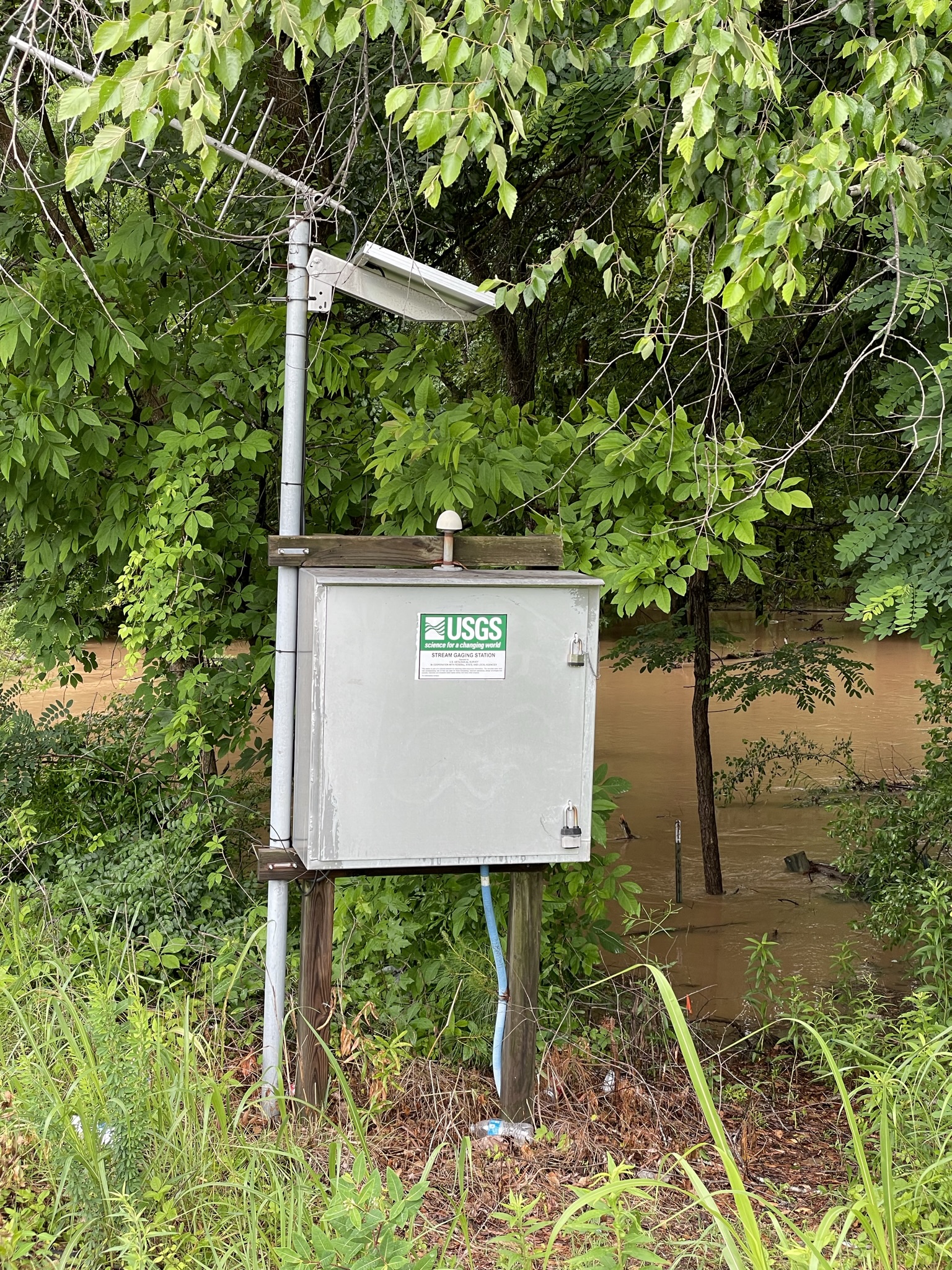
Sensor Networks

In-situ sensor networks are used to collect data in the environment. Common use cases incldue weather stations, flood gauges, and air quality sensors.

Mobile Devices

Mobile devices are used to collect data in the field. Common use cases include GPS data, photos, and field observations.

Coordinate Reference Systems (CRS)

Coordinate reference systems (CRS) are used to specify the location of a point on the Earth’s surface.

Geodetic (Geographic) coordinate systems are used to specify the location of a point on the Earth’s surface using latitude and longitude (units degree:minutes:seconds).

Example:

-78.0, 35.0 (Durham, NC)

Use Case:

GPS coordinates
Large regions
Data Exchange

The most common CRS is the WGS84, which is used by GPS systems.

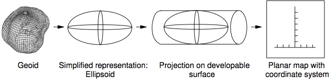
Projected coordinate systems are used to represent the Earth’s surface on a flat map.

Projected coordinate systems are a type of CRS that is used to represent the Earth’s surface on a flat map. Each version uses a different mathematical model to transform the Earth’s three-dimensional surface into a two-dimensional plane. The choice of a projected coordinate system depends on the region of interest and the purpose of the map.

Example Developable Surfaces: - Cylindrical - Conic - azimuthal

Types of distortion: - Conformal - Equal Area - Equidistant

In North Carolina,NAD83 North Carolina State Plane (EPSG: 3358) is a commonly used projected coordinate system. It uses the Lambert Conformal Conic projection and has units of meters. You can find other various of CRS at epsg.io that can be used for different regions of the world.

Web Mapping & Pseudo-Mercator

Pseudo-Mercator (EPSG: 3857) is a projected coordinate system that is used by web mapping services such as Google Maps, OpenStreetMap, and Bing Maps. It uses the Mercator projection and has units of meters.

Even though it is widely used for web mapping, it is not recommend for professional work because it has a high level of distortion at high latitudes and considers the Earth as a perfect sphere instead of an geoid.

You can see for yourself the distortion of the Mercator projection by using the The true size website.

Learn More Learn more about Map projection transitions Look up CRS at epsg.io

Introduction GRASS GIS

What is a Geospatial Processing Engine?

A geospatial processing engine is a tool that allows to efficiently manipulate geospatial data through the development of scriptable geoprocesing workflows. Geoprocessing engines can be used on a local machine, distributed on the cloud, or on HPC (high performance computing) clusters (i.e., super computers).

With GRASS you can effiently process geospatial data with over 800 tools or develop your own models or tools using its C and Python APIs.

The tools are prefixed to reflect the type of data they are designe to work with.

Category	Description	Examples
*Display (d.)**	display commands for graphical screen output	`d.rast`, `d.vect`
*General (g.)**	general file management commands	`g.list`, `g.copy`
*Raster (r.)**	raster processing commands	`r.slope.aspect`, `r.mapcalc`
*Vector (v.)**	vector processing commands	`v.digit`, `v.to.rast`
*Imagery (i.)**	image processing commands	`i.atcorr`, `i.pansharpen`
*Database (db.)**	database commands (SQLite, Postgresql, etc..)	`db.select`, `db.in.ogr`
*Raster 3D (r3.)**	3D raster (voxel) processing commands	`r3.mapcalc`, `r3.gwflow`
*Temporal (t.)**	spatio-temporal data processing commands	`t.rast.aggregate`, `t.rast.series`
*Miscellaneous (m.)**	miscellaneous commands	`m.proj`, `m.nviz.image`

GRASS GIS Reference Manual

GRASS GIS Projects and Mapsets

In GRASS a project resprests a group of data that is all in the same CRS. Each project can have a collection of subprojects called mapsets. A mapset contains map layers in raster or vector format. Each project has a PERMANENT mapset that is used to store the original data.

Learn More.

Coordinate Reference Systems in GRASS GIS

Every project in GRASS GIS has a CRS. You can view the CRS of a project using the g.proj tool.

We are currently in the nc_basic_spm_grass7 project, which uses the NAD83 / North Carolina (meters) coordinate reference system (EPSG:3358).

Create a new GRASS GIS Mapset

Here we will use the GRASS GIS shell command to create a new GRASS GIS mapset. The ! is used to run shell commands in a Jupyter notebook. The grass command is used to start GRASS GIS and the -c flag is used to create a new GRASS GIS mapset and -e tells the command to exit after it finishes.

# ! means that we are running a command in the shell
!grass -e -c ./grassdata/nc_basic_spm_grass7/tutorial

GRASS GIS with Python

GRASS GIS has two core libraries for working with geospatial data in Python:

grass.script - Python library for working with GRASS GIS modules
grass.pygrass - Python library for working with GRASS GIS data structures

We will use the grass.script as gs library to perform geoprocessing tasks in this workshop.

For interaction with Jupiter notebooks, we will use grass.jupyter as gj to display maps and other outputs.

GRASS Python Environment Setup

To use GRASS GIS in Python, we need to set the GISBASE environment variable to the location of the GRASS GIS installation. We also need to add the GRASS GIS Python library to the Python path.

import os
import subprocess
import sys
import matplotlib.pyplot as plt
import pandas as pd
from IPython.display import display

# Switch to the home directory
# os.chdir(os.path.expanduser("~")) # Colab only

# Ask GRASS GIS where its Python packages are.
sys.path.append(
    subprocess.check_output(["grass", "--config", "python_path"], text=True).strip()
)

# Import the GRASS GIS packages we need.
import grass.script as gs

# Import GRASS Jupyter
import grass.jupyter as gj

GRASS GIS Session

With our Python environment setup we can start a GRASS GIS session using the gj.init function. Here we pass the the path to our project/mapset (nc_basic_spm_grass7/tutorial). This will allow us to exectute GRASS GIS commands in Python in the tutorial mapset.

# Start a GRASS session
session = gj.init("./grassdata", "nc_basic_spm_grass7", "tutorial")

Let’s look at the details of the project CRS using the g.proj command.

gs.run_command("g.proj", flags="g")

name=Lambert Conformal Conic
proj=lcc
datum=nad83
a=6378137.0
es=0.006694380022900787
lat_1=36.16666666666666
lat_2=34.33333333333334
lat_0=33.75
lon_0=-79
x_0=609601.22
y_0=0
no_defs=defined
srid=EPSG:3358
unit=Meter
units=Meters
meters=1

GRASS GIS Layers

The g.list command or the Python helper function gs.list_grouped let us list what data we have able in our project. We can search by data type and filter the data by mapset.

Here we will list all the raster and vector data in the PERMANENT mapset.

gs.list_grouped(type="raster")['PERMANENT']

['basins',
 'elevation',
 'elevation_shade',
 'geology',
 'lakes',
 'landuse',
 'soils']

gs.list_grouped(type="vector")['PERMANENT']

['boundary_region',
 'boundary_state',
 'census',
 'elev_points',
 'firestations',
 'geology',
 'geonames',
 'hospitals',
 'points_of_interest',
 'railroads',
 'roadsmajor',
 'schools',
 'streams',
 'streets',
 'zipcodes']

Our project has 7 raster and 15 layers for us to examine. However, we must first define computational region before we can work with the data.

Computational Region

In GRASS GIS the region or computational region defines the spatial scale used during computation. Spatial scale reprents the resolution (i.e., grain) of each pixel and the total extent (i.e., area) of the raster.

The computational region impacts your analytical results and the amount of time it takes to process data. You can change the spatial scale by defining regions extent and upscaling (finer data, increased resolution) or downscale (coarser data, decrease resolution) the data.

We can view and set the computational region using the g.region command or the pygrass function gs.region. The raster flag is used to set the region to the extent of a raster layer. The res flag is used to set the resolution of the region.

First, let’s view the current computational region.

# Prints the current computational region
gs.region()

{'projection': 99,
 'zone': 0,
 'n': 228500.0,
 's': 215000.0,
 'w': 630000.0,
 'e': 645000.0,
 'nsres': 10.0,
 'ewres': 10.0,
 'rows': 1350,
 'cols': 1500,
 'cells': 2025000}

Now set the computational region to the spatial scale of the elevation raster layer. The elevation raster data is a Digital Elevation Model (DEM) of the area around Wake County, North Carolina.

gs.region("elevation")

{'projection': 99,
 'zone': 0,
 'n': 228500.0,
 's': 215000.0,
 'w': 630000.0,
 'e': 645000.0,
 't': 1.0,
 'b': 0.0,
 'nsres': 10.0,
 'nsres3': 10.0,
 'ewres': 10.0,
 'ewres3': 10.0,
 'tbres': 1.0,
 'rows': 1350,
 'rows3': 1350,
 'cols': 1500,
 'cols3': 1500,
 'depths': 1,
 'cells': 2025000,
 'cells3': 2025000}

Adjusting the Computational Region

With raster data we can use spatial interpolation to resample our data.

Note: We use different methods for continuous and discrete spatial data.

Here the elevation raster layer is resampled using bliniear interpolation so that each cell has a resolution of 250m, 500m, and 1000m using r.resample.interp.

# Set the computational region to the extent of the elevation raster layer with a resolution of 250m making sure to align the region with the rasters grid
gs.run_command('g.region', raster='elevation', res=250, flags='a')

# Resample the elevation raster layer to 250m resolution using bilinear interpolation
gs.run_command('r.resamp.interp', input='elevation', output='elevation_250m', method='bilinear')

What impact does resampling have on our evelation data?

Let’s look at what happends when we resample discete raster data like landuse.

# Set the computational region to the extent of the landuse raster layer with a resolution of 250m making sure to align the region with the rasters grid
gs.run_command('g.region', raster='landuse', res=250, flags='a')

# Resample the landuse raster layer to 250m resolution using nearest neighbor interpolation
gs.run_command('r.resamp.interp', input='landuse', output='landuse_250m', method='nearest')

Processing Data

Now that we have set the computational region, we can perform geoprocessing tasks on the data. Here we will use the r.slope.aspect tool to calculate the slope and aspect of the elevation raster layer by running the tool with gs.run_command. The run_command should be used when you do not need a return value from the tool.

gs.run_command("r.slope.aspect", elevation="elevation", slope="slope", aspect="aspect")

The slope represents the steepest slope (maximum gradient) angle in degrees from the horizontal plane. The aspect represents the direction that the slope faces.

We can create a DataFrame of the univariate statistics from the slope layer using the r.univar tool by running the tool with gs.parse_command and setting the format to json.

import json

slope_stats_json = gs.read_command("r.univar", map="slope", format="json", flags="e")
slope_stats_dict = json.loads(slope_stats_json)
df_slope = pd.DataFrame(slope_stats_dict)
df_slope = df_slope.T.reset_index()
df_slope.columns = ["statistic", "value"]
df_slope.head(15)

	statistic	value
0	n	2019304
1	null_cells	5696
2	cells	2025000
3	min	0
4	max	38.689392
5	range	38.689392
6	mean	3.864522
7	mean_of_abs	3.864522
8	stddev	3.007914
9	variance	9.047547
10	coeff_var	77.834045
11	sum	7803645.553885
12	first_quartile	1.854639
13	median	3.215121
14	third_quartile	5.024211

Date Visualization

Maps

Map layers can be displayed using the GRASS Jupyter function gj.Map to create a map object. Map objects can use GRASS display tools like d.rast and d.vect to visualize vector and raster map layers.

dem_map = gj.Map(height=600, width=800, filename="static_map.png") # Create a map object
dem_map.d_rast(map="elevation") # Add the raster map to the map object
dem_map.d_vect(map="roadsmajor", color="black") # Add the vector map to the map object

# Add a raster legend
# dem_map.d_legend(
#     raster="elevation",
#     at=(5,40,11,14),
#     title="Elevation (m)",
#     font="sans",
#     flags="b"
# ) 
# dem_map.d_barscale(at=(50,7), flags="n") # Add a scale bar to the map
dem_map.show() # Display the map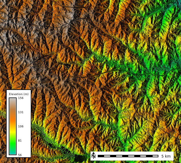

Let’s overlay the elevation data over the aspect to see how the terrain looks with shaded relief.

dem_map = gj.Map(height=600, width=800, filename="relief_map.png") # Create a map object
dem_map.d_shade(color="elevation", shade="aspect") # Add a shaded relief map
dem_map.d_vect(map="roadsmajor", color="black") # Add the vector map to the map object

# Add a raster legend
dem_map.d_legend(
    raster="elevation",
    at=(5,40,11,14),
    title="Elevation (m)",
    font="sans",
    flags="b"
) 
dem_map.d_barscale(at=(50,7), flags="n") # Add a scale bar to the map
dem_map.show() # Display the map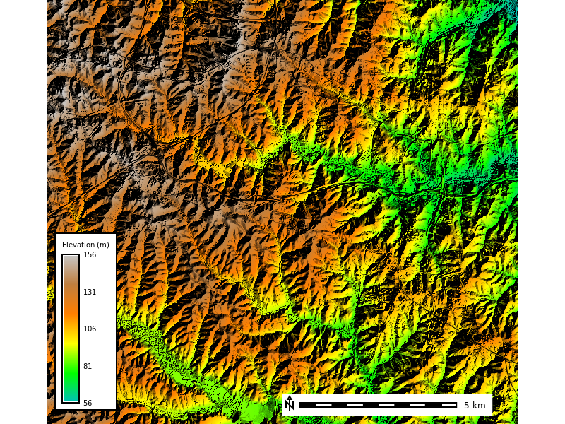

We can also change the color scheme of our map layers using the r.colors tool. Here we will change the color scheme of the aspect layer to aspectcolr.

gs.run_command("r.colors", map="aspect", color="aspectcolr")

Plots

GRASS also provide a number of build in plotting options for raster data.

Here we will use the d.histogram tool to create a histogram of the elevation raster layer.

hist_plot = gj.Map(font="sans", height=600, width=800, filename="jupyterintro_hist_plot.png")
hist_plot.d_histogram(map="elevation")
hist_plot.show()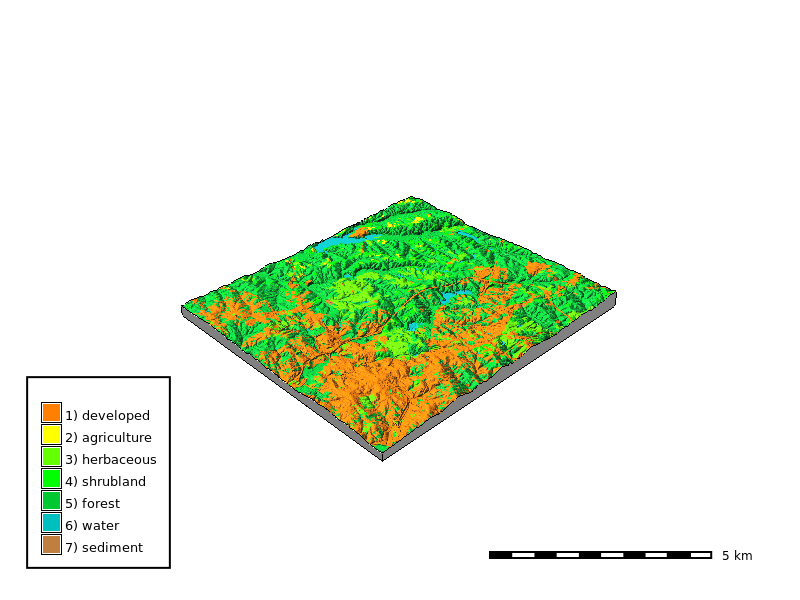

We can also make polar plots. Here we make a polar plot of the aspect raster layer.

polar_plot = gj.Map(font="sans", height=600, width=800, filename="jupyterintro_polar_plot.png")
polar_plot.d_polar(map="aspect", undef=0)
polar_plot.show()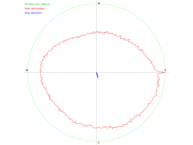

dem_shade_map = gj.Map() # Create a map object
dem_shade_map.d_shade(color="aspect", shade="aspect") # Add a shaded relief map
dem_shade_map.d_legend(raster="aspect", at=(5,50,5,9), flags="b") # Add a raster legend
dem_shade_map.d_barscale(at=(50,7,1,1), flags="n") # Add a scale bar to the map
dem_shade_map.show() # Display the map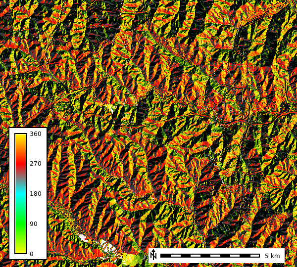

3D Maps

GRASS GIS can also create 3D maps using the nviz tool. The nviz tool allows you to visualize raster and vector data in 3D space. Here we will create a 3D map of the elevation data overlayed with the landuse data.

elevation_3dmap = gj.Map3D(height=600, width=800, filename="jupyterintro_3D_map.png")
# Full list of options m.nviz.image
# https://grass.osgeo.org/grass-stable/manuals/m.nviz.image.html
elevation_3dmap.render(
    elevation_map="elevation",
    color_map="landuse",
    perspective=35,
    height=5000,
    resolution_fine=1,
    zexag=5,
    fringe=['ne','nw','sw','se'],
    fringe_elevation=10,
    arrow_position=[100,50],
)
elevation_3dmap.overlay.d_barscale(at=(60,10))
elevation_3dmap.overlay.d_legend(raster="landuse", at=(5,35,5,9), flags="b")
elevation_3dmap.show()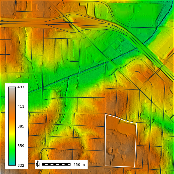

Web Maps

Interactive web maps can be created using the GRASS Jupyter function gj.InteractiveMap. The InteractiveMap map feature uses either Folium or ipyleaflet as a backend to render the web map within Jupyter.

We will create an interactive web map of the elevation, aspect, slope, and roadsmajor data using the ipyleaflet backend. The ipyleaflet backend allows you to query map layers, add new vector layers, and interactively set the computational region.

# Create a new InteractiveMap object
elevation_map = gj.InteractiveMap(width=800, height=600)

# Add raster and vector layers to the map
elevation_map.add_raster("aspect", opacity=0.5)
elevation_map.add_raster("elevation", opacity=0.7)
elevation_map.add_vector("roadsmajor", color="black")

# Display the map
display(elevation_map.show())

NCSSM Analysis

We will now create a basic workflow for a geoprocessing task using the ncssm data. The ncssm data is a subset of the nc_basic_spm_grass7 project that contains data around the North Carolina School of Science and Mathematics (NCSSM) in Durham, North Carolina.

To begin we must first create a GRASS session in the ncssm mapset (downloaded at the begining of the workshop) and set the computational region to the extent of the ncssm_be_1m raster layer. The ncssm_be_1m raster data is a \(1 m\) Digital Terrain Model (DTM) of the area around NCSSM.

gj.init("./grassdata/nc_basic_spm_grass7/ncssm")
gs.run_command("g.region", raster="ncssm_be_1m", res=1, flags="ap")

projection: 99 (Lambert Conformal Conic)
zone:       0
datum:      nad83
ellipsoid:  a=6378137 es=0.006694380022900787
north:      252984
south:      251460
west:       615696
east:       617223
nsres:      1
ewres:      1
rows:       1524
cols:       1527
cells:      2327148

Now we will compute the relief map for our visualizations using the r.relief tool and will display the ncssm_be_1m layer.

gs.run_command(
    "r.relief",
    input="ncssm_be_1m",
    output="relief",
    altitude=45,
    scale=1,
    overwrite=True
)

ncssm_map = gj.Map()
ncssm_map.d_shade(color="ncssm_be_1m", shade="relief")
ncssm_map.d_vect(map="ncssm", fill_color="none", color="white", width=2)
ncssm_map.d_vect(map="roads")
ncssm_map.d_legend(raster="ncssm_be_1m", at=(5,50,5,9), flags="b")
ncssm_map.d_barscale(at=(20,8), flags="n", length=250)
ncssm_map.show()

Let’s view what the ncssm project has to offer.

# In this cell list all of the raster and vector data available in the ncssm mapset

# Add your code here

Now let’s look at the ncssm project data. In the cell below add a raster and vector layer to the ncssm_map object.

ncssm_map = gj.Map() # Create a map object

# Add a raster map here



# Add a vector map here


ncssm_map.d_barscale(at=(10,7), flags="n") # Add a scale bar to the map
ncssm_map.show() # Display the map

Let’s look at the the NAIP (National Agriculture Imagery Program) data in the ncssm project. The NAIP data is a high resolution aerial imagery dataset that is used for land cover classification, change detection, and other geospatial analysis tasks. It is available at a spatial resolution of \(1m\) and \(0.5m\) and has a spatial extent of the United States and 4 spectoral bands (RGB, NIR) for most years.

map_rgb = gj.Map()
map_rgb.d_rgb(red="naip2022.blue", green="naip2022.green", blue="naip2022.red")
map_rgb.d_vect(map="ncssm", fill_color="none", color="white", width=2)
map_rgb.d_barscale(at=(10,7), flags="n")
map_rgb.show()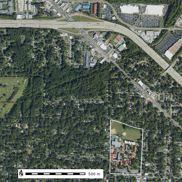

map = gj.Map()
map.d_rgb(red="naip2022.nir", green="naip2022.nir", blue="naip2022.red")
map.d_vect(map="ncssm", fill_color="none", color="white", width=2)
map.d_barscale(at=(10,7), flags="n")
map.show()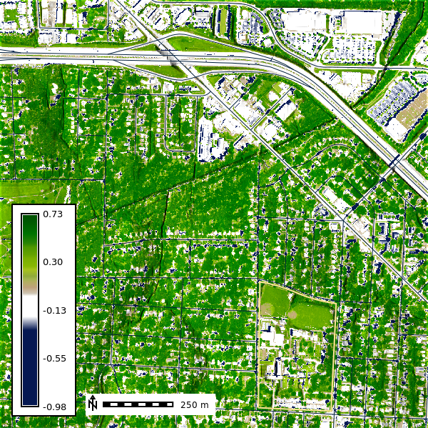

Play around with different band combinations to see how the data looks. Do different combinations highlight different features in the data?

import ipywidgets as widgets
from IPython.display import display, clear_output

# List of available bands
bands = ["naip2022.red", "naip2022.green", "naip2022.blue", "naip2022.nir"]

selected_band_1 = bands[0]
selected_band_2 = bands[1]
selected_band_3 = bands[2]

def display_map(selected_band_1, selected_band_2, selected_band_3):
    map = gj.Map()
    map.d_rgb(red=selected_band_1, green=selected_band_2, blue=selected_band_3)
    map.d_vect(map="ncssm", fill_color="none", color="white", width=2)
    map.d_barscale(at=(10,7), flags="n")
    return map.show()

# Display the initial map
the_map = display_map(selected_band_1, selected_band_2, selected_band_3)

# Create dropdown widgets
band_selector1 = widgets.Dropdown(
    options=bands,
    value=selected_band_1,
    description='Band: 1',
    disabled=False,
)

band_selector2 = widgets.Dropdown(
    options=bands,
    value=selected_band_2,
    description='Band: 2',
    disabled=False,
)

band_selector3 = widgets.Dropdown(
    options=bands,
    value=selected_band_3,
    description='Band: 3',
    disabled=False,
)

# Arrange the dropdown widgets horizontally
hbox = widgets.HBox([band_selector1, band_selector2, band_selector3])

# Function to handle changes in dropdowns
def on_band_change(change):
    global selected_band_1, selected_band_2, selected_band_3
    if change['owner'] == band_selector1:
        selected_band_1 = change['new']
    elif change['owner'] == band_selector2:
        selected_band_2 = change['new']
    elif change['owner'] == band_selector3:
        selected_band_3 = change['new']
    clear_output(wait=True)
    display(hbox)
    display(display_map(selected_band_1, selected_band_2, selected_band_3))


# Observe changes in dropdowns
band_selector1.observe(on_band_change, names='value')
band_selector2.observe(on_band_change, names='value')
band_selector3.observe(on_band_change, names='value')

# Display the dropdown widgets and the map
display(hbox, the_map)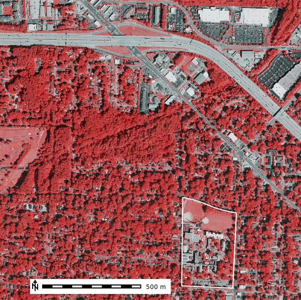

NDVI (Normalized Difference Vegetation Index)

NDVI is a simple calculation that measure chlorophyll absorbtion in plants. It utilizes the Red and Near-Infrared (NIR) light to produce an index between -1 and 1 where 1 represents healthy vegetation and values less than or equal to 0 represent bare earth or other forms of imperious surface.

\[ NDVI = \frac{(NIR - Red)}{(NIR + Red)} \]

gs.run_command(
    "i.vi",
    viname="ndvi",
    red="naip2022.red",
    nir="naip2022.nir",
    output="naip2022_ndvi"
)

Let’s viusalize the NDVI for the area around NCSSM.

ndvi_map = gj.Map()
ndvi_map.d_shade(color="naip2022_ndvi", shade="relief", brighten=30)
ndvi_map.d_vect(map="ncssm", fill_color="none", color="#FFE599", width=2)
ndvi_map.d_vect(map="roads")
ndvi_map.d_barscale(at=(20,8), flags="n", length=250)
ndvi_map.d_legend(raster="naip2022_ndvi", at=(5,50,5,9), flags="b")
ndvi_map.show()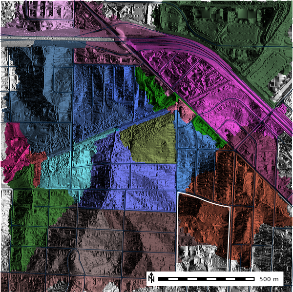

Let’s see what the NDVI looks like in 3D.

Does not work in Google Colab

elevation_3dmap = gj.Map3D(use_region=False)
# Full list of options m.nviz.image
# https://grass.osgeo.org/grass-stable/manuals/m.nviz.image.html
elevation_3dmap.render(
    elevation_map="ncssm_1m",
    color_map="naip2022_ndvi",
    perspective=30,
    height=3000,
    resolution_fine=1,
    zexag=1,
    fringe=['ne','nw','sw','se'],
    fringe_elevation=200,
    arrow_position=[100,50],
)
elevation_3dmap.show()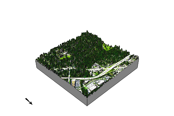

Let now calcuate the average NDVI in the subwatersheds around NCSSM. To do this we will first need to compute the subwatersheds using the r.watershed tool and then compute the average NDVI in each subwatershed using the r.stats.zonal tool.

The r.watershed tool will calculate the flow direction, flow accumulation, stream network, and basins for a given threshold. The threshold is the minimum number of cells of an exterior watershed basin. An exterior watershed basin is an area where rainwater collects and flows out of the edge of a map or region, like water running off the edge of a table.

In practicle terms, the threshold controls the size of the generated basins and stream network. A lower threshold will generate more basins and a higher threshold will generate fewer basins.

gs.run_command(
    "r.watershed", 
    elevation="ncssm_be_1m", 
    threshold=50000,
    drainage="direction50k",
    basin="basins50k", 
    stream="streams50k", 
    memory=300
)

Let’s now view the basins50k map layer.

basins10k_map = gj.Map()
basins10k_map.d_shade(color="basins50k", shade="aspect")
basins10k_map.d_vect(map="ncssm", fill_color="none", color="white", width=2)
basins10k_map.d_vect(map="roads")
basins10k_map.d_barscale(at=(50,7,1,1), flags="n")
basins10k_map.show()

For each basin we will calculate the average NDVI using the r.stats.zonal tool. The r.stats.zonal tool calculates univariate statistics for raster map layers within zones defined by the categories in the basin map. Here we will calculate the average NDVI in each basin using the average (mean) flag.

gs.run_command(
    "r.stats.zonal",
    base="basins50k",
    cover="naip2022_ndvi",
    method="average",
    output="basins50k_ndvi_avg", 
    flags="c"
)

We can convert our raster basin map to a vector layer to help with visulization and analysis. The r.to.vect tool converts raster map layers to vector map layers. Here we will convert the basins50k raster layer to a vector layer called basins50k.

gs.run_command("r.to.vect", input="basins50k", output="basins50k", type="area", flags="v")

# Change the map color
gs.run_command("r.colors", map="basins50k_ndvi_avg", color="ndvi", flags="")

basins10k_map = gj.Map()
basins10k_map.d_shade(color="basins50k_ndvi_avg", shade="aspect")
basins10k_map.d_vect(map="ncssm", fill_color="none", color="#FFE599", width=2)
basins10k_map.d_vect(map="roads")
basins10k_map.d_vect(map="basins50k", color="white", fill_color="none", width=2)
basins10k_map.d_barscale(at=(20,8), flags="n", length=250)
basins10k_map.d_legend(raster="naip2022_ndvi", at=(5,50,5,9), flags="b")
basins10k_map.show()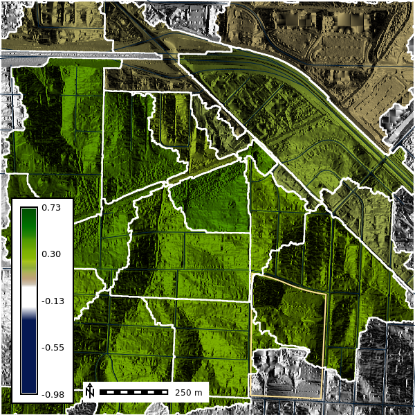

Estimate Flood Innundation

Let’s estimate the flood inundation for the area around NCSSM using the Height Above Nearest Drainage methodology (A.D. Nobre, 2011). First need to install two GRASS addons r.stream.distance and r.lake.series to calculate the distance to the nearest stream and create a flood inundation map.

gs.run_command("g.extension", extension="r.stream.distance")
gs.run_command("g.extension", extension="r.lake.series")

Your branch is up to date with 'origin/grass8'.
Your branch is up to date with 'origin/grass8'.

Here we will simulate the flood inundation extent starting from \(0 m\) to \(5 m\) above the nearest stream.

gs.run_command("r.stream.distance", stream_rast="streams50k", direction="direction50k", elevation="ncssm_be_1m", method="downstream", difference="above_stream")
gs.run_command("r.lake.series", elevation="above_stream", start_water_level=0, end_water_level=5, water_level_step=0.5, output="flooding", seed="streams50k")

We can visulize the flood event from using the time series of the flood stages using gj.TimeSeries.

flood_map = gj.TimeSeriesMap()
flood_map.d_rast(map="naip_2022_rgb")
flood_map.d_vect(map="ncssm", fill_color="none", color="white", width=2)
flood_map.d_vect(map="roads")
flood_map.add_raster_series("flooding")
flood_map.d_legend()
# flood_map.save("output/flooding.gif")
flood_map.show()

We can further analysze our results by looking at the r.univar statistics of the flood inundation layers.

import io

flood_output = gs.read_command("t.rast.univar", input="flooding", separator="comma")
df_flood = pd.read_csv(io.StringIO(flood_output), sep=",")
df_flood.head()

	id	semantic_label	start	end	mean	min	max	mean_of_abs	stddev	variance	coeff_var	sum	null_cells	cells	non_null_cells
0	flooding_0.0@ncssm	NaN	1	NaN	1.856766	0.000031	9.473022	1.856766	2.171698	4.716271	116.961330	30707.188751	2310610	16538	16538
1	flooding_0.5@ncssm	NaN	31	NaN	0.869660	0.000031	9.973022	0.869660	1.401108	1.963104	161.109846	62770.329803	2254970	72178	72178
2	flooding_1.0@ncssm	NaN	61	NaN	0.941503	0.000031	10.473022	0.941503	1.222776	1.495182	129.874969	111666.929962	2208543	118605	118605
3	flooding_1.5@ncssm	NaN	91	NaN	1.155722	0.000031	10.973022	1.155722	1.179905	1.392175	102.092457	181055.370209	2170488	156660	156660
4	flooding_2.0@ncssm	NaN	121	NaN	1.412721	0.000031	11.473022	1.412721	1.196605	1.431864	84.702150	268414.241577	2137150	189998	189998

ax = df_flood.plot(x="start", y="mean", title="Mean flooding depth over time", label="Mean")
df_flood.plot(x="start", y="min", ax=ax, style='--', label="Min", color='gray')
df_flood.plot(x="start", y="max", ax=ax, style='--', label="Max", color='gray')
ax.fill_between(df_flood["start"], df_flood["min"], df_flood["max"], color='gray', alpha=0.3)
plt.ylabel("Flooding depth (m)")
plt.xlabel("Time (minutes)")
plt.show()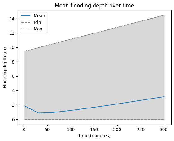

df_flood['extent_km2'] = df_flood['cells'] * 0.000001
ax = df_flood.plot(x="start", y="extent_km2", title="Inundation Extent", label="Extent")
ax.axhline(y=2327148 * 0.000001, color='gray', linestyle='--', label='Study Area Extent')
plt.legend()
plt.ylabel("Inundation Extent (km2)")
plt.xlabel("Time (minutes)")
plt.show()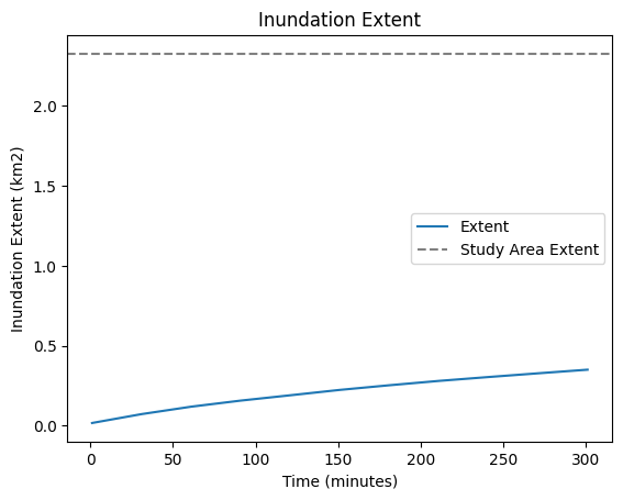

Interactive Estimated Flood Inundation Map

flood_map = gj.InteractiveMap(height=800,width=800)
flood_map.add_raster("naip_2022_rgb")
flood_map.add_raster("flooding_5.0")
flood_map.add_layer_control()
display(flood_map.show())

Export Map as HTML

flood_map.save(filename="./output/index.html")

Create a new Project (Location and Mapset)

Create a new subproject (i.e. Mapset)

This example uses a temprary directory to create a new project call myfirstproject with the EPSG:3358 CRS.

from pathlib import Path
import tempfile

tempdir = tempfile.TemporaryDirectory()

gs.create_project(path=tempdir, name="myfirstproject", epsg="3358")

Start a new GRASS GIS session in the new subproject

gj.init(Path(tempdir.name), "myfirstproject")

Local Data Resources

Where can I get my own geospatial data?

North Carolina Online Data Portals

# Point Data
hospitals = "https://webgis2.durhamnc.gov/server/rest/services/PublicServices/Community/MapServer/0/query?outFields=*&where=1%3D1f=geojson"
schools = "https://webgis2.durhamnc.gov/server/rest/services/PublicServices/Education/MapServer/0/query?outFields=*&where=1%3D1&f=geojson"

# Line Data
roads = "https://webgis2.durhamnc.gov/server/rest/services/PublicServices/Transportation/MapServer/6/query?outFields=*&where=1%3D1f=geojson"
greenways = "https://webgis2.durhamnc.gov/server/rest/services/ProjectServices/Trans_ExistingFutureBikePedFacilities/MapServer/1/query?outFields=*&where=1%3D1f=geojson"
sidewalks = "https://webgis2.durhamnc.gov/server/rest/services/PublicServices/Community/MapServer/5/query?outFields=*&where=1%3D1f=geojson"

# Polygon Datahttps://earth.nullschool.net
zipcodes = "https://webgis2.durhamnc.gov/server/rest/services/PublicServices/Administrative/MapServer/0/query?outFields=*&where=1%3D1f=geojson"
county_boundary = "https://webgis2.durhamnc.gov/server/rest/services/PublicServices/Administrative/MapServer/2/query?outFields=*&where=1%3D1f=geojson"
durham_city_boundary = "https://webgis2.durhamnc.gov/server/rest/services/PublicServices/Administrative/MapServer/1/query?outFields=*&where=1%3D1f=geojson"
school_districts = "https://webgis2.durhamnc.gov/server/rest/services/PublicServices/Education/MapServer/1/query?outFields=*&where=1%3D1f=geojson"

!v.import --help

Imports vector data into a GRASS vector map using OGR library and reprojects on the fly.

Usage:
 v.import [-flo] input=string [layer=string[,string,...]] [output=name]
   [extent=string] [encoding=string] [snap=value] [epsg=value]
   [datum_trans=value] [--overwrite] [--help] [--verbose] [--quiet]
   [--ui]

Flags:
  -f   List supported OGR formats and exit
  -l   List available OGR layers in data source and exit
  -o   Override projection check (use current location's projection)

Parameters:
        input   Name of OGR datasource to be imported
        layer   OGR layer name. If not given, all available layers are imported
       output   Name for output vector map (default: input)
       extent   Output vector map extent
                options: input,region
                default: input
     encoding   Encoding value for attribute data
         snap   Snapping threshold for boundaries (map units)
                default: -1
         epsg   EPSG projection code
                options: 1-1000000
  datum_trans   Index number of datum transform parameters
                options: -1-100

!r.import --help

Imports raster data into a GRASS raster map using GDAL library and reprojects on the fly.

Usage:
 r.import [-enlo] input=name [band=value[,value,...]]
   [memory=memory in MB] [output=name] [resample=string] [extent=string]
   [resolution=string] [resolution_value=value] [title=phrase]
   [--overwrite] [--help] [--verbose] [--quiet] [--ui]

Flags:
  -e   Estimate resolution only
  -n   Do not perform region cropping optimization
  -l   Force Lat/Lon maps to fit into geographic coordinates (90N,S; 180E,W)
  -o   Override projection check (use current location's projection)

Parameters:
             input   Name of GDAL dataset to be imported
              band   Input band(s) to select (default is all bands)
            memory   Maximum memory to be used (in MB)
                     default: 300
            output   Name for output raster map
          resample   Resampling method to use for reprojection
                     options: nearest,bilinear,bicubic,lanczos,bilinear_f,
                              bicubic_f,lanczos_f
                     default: nearest
            extent   Output raster map extent
                     options: input,region
                     default: input
        resolution   Resolution of output raster map (default: estimated)
                     options: estimated,value,region
                     default: estimated
  resolution_value   Resolution of output raster map (use with option resolution=value)
             title   Title for resultant raster map

Install Add-Ons

Add-On Index

!g.extension --help

Maintains GRASS Addons extensions in local GRASS installation.

Usage:
 g.extension [-lcgasdifto] extension=name operation=string [url=url]
   [prefix=path] [proxy=proxy[,proxy,...]] [branch=branch] [--help]
   [--verbose] [--quiet] [--ui]

Flags:
  -l   List available extensions in the official GRASS GIS Addons repository
  -c   List available extensions in the official GRASS GIS Addons repository including module description
  -g   List available extensions in the official GRASS GIS Addons repository (shell script style)
  -a   List locally installed extensions
  -s   Install system-wide (may need system administrator rights)
  -d   Download source code and exit
  -i   Do not install new extension, just compile it
  -f   Force removal when uninstalling extension (operation=remove)
  -t   Operate on toolboxes instead of single modules (experimental)
  -o   url refers to a fork of the official extension repository

Parameters:
  extension   Name of extension to install or remove
  operation   Operation to be performed
              options: add,remove
              default: add
        url   URL or directory to get the extension from (supported only on Linux and Mac)
     prefix   Prefix where to install extension (ignored when flag -s is given)
              default: $GRASS_ADDON_BASE
      proxy   Set the proxy with: "http=<value>,ftp=<value>"
     branch   Specific branch to fetch addon from (only used when fetching from git)