---
title: "Watershed analysis with r.watershed"
description: "Delineate stream networks and watersheds from a DEM with r.watershed in GRASS, and see how the threshold and cell size affect the result."
author: "Corey T. White"
date: "2026-09-03"
date-modified: today
image: images/cover.png
categories: [grass, hydrology, terrain, watershed, tutorial]
draft: false
page-layout: full
title-block-banner: true
format:
html:
toc: true
toc-depth: 3
code-copy: true
code-fold: true
code-summary: "Show code"
code-tools: true
lightbox: true
other-links:
- text: r.watershed manual
href: https://grass.osgeo.org/grass-stable/manuals/r.watershed.html
- text: GRASS sample data
href: https://grass.osgeo.org/download/data/
engine: jupyter
jupyter: python3
execute:
enabled: true
eval: true
freeze: true
cache: false
keep-ipynb: false
---
```{=html}
<style>
.plg-watershed { max-width: 640px; margin: 1.5rem auto; }
.plg-watershed svg { width: 100%; height: auto; display: block; }
.plg-watershed .plg-caption {
font-size: 0.9rem; color: #4e4d4c; text-align: center; margin: 0.5rem 0 0;
}
.plg-watershed .drop { opacity: 0; }
.plg-watershed .divide { opacity: 0.35; }
@media (prefers-reduced-motion: no-preference) {
.plg-watershed .drop { animation: plg-slide 5s ease-in infinite; }
.plg-watershed .drop.right { animation-name: plg-slide-right; }
.plg-watershed .drop.d2 { animation-delay: 0.9s; }
.plg-watershed .drop.d3 { animation-delay: 1.8s; }
.plg-watershed .divide { animation: plg-fade 5s linear infinite; }
@keyframes plg-slide {
0% { transform: translate(0, -30px); opacity: 0; }
8% { transform: translate(0, 0); opacity: 1; }
55% { transform: translate(-235px, 81px); opacity: 1; }
62% { transform: translate(-235px, 81px); opacity: 0; }
100% { transform: translate(-235px, 81px); opacity: 0; }
}
@keyframes plg-slide-right {
0% { transform: translate(0, -30px); opacity: 0; }
8% { transform: translate(0, 0); opacity: 1; }
55% { transform: translate(235px, 81px); opacity: 1; }
62% { transform: translate(235px, 81px); opacity: 0; }
100% { transform: translate(235px, 81px); opacity: 0; }
}
@keyframes plg-fade {
0%, 50% { opacity: 0; }
65%, 100% { opacity: 1; }
}
}
@media (prefers-reduced-motion: reduce) {
.plg-watershed .drop { opacity: 1; }
.plg-watershed .divide { opacity: 1; }
}
</style>
```
This guide delineates stream networks and watersheds from a digital elevation
model using
[`r.watershed`](https://grass.osgeo.org/grass-stable/manuals/r.watershed.html)
in GRASS, then looks at how the threshold and the cell size affect the result.
For a broader treatment of terrain analysis in GRASS, including watershed
analysis alongside slope, curvature, solar radiation, and visibility, see the
Geomorphometry in GRASS chapter (White et al., 2026).
::: {.callout-note}
## Who this is for
This guide assumes some GIS experience but no experience with GRASS. If you
have never used GRASS, the
[first-time users page](https://grass.osgeo.org/learn/newcomers/) is a good
place to start.
:::
## What is a watershed
Rain that lands on a hillside runs downhill until it reaches a low point and
leaves the area, through a stream, a lake, or the edge of the map. Call that
low point an exit. A watershed is the area whose rain leaves through the same
exit. The boundary between two watersheds is called a divide. Rain falling on
one side of a divide runs to one exit, and rain on the other side runs to
another.
`r.watershed` finds watersheds on a grid of elevation cells. For each cell it
works out which neighbor the water flows to, follows those links downhill, and
groups cells that end up at the same exit. The divides are the boundaries
between those groups.
```{=html}
<figure class="plg-watershed">
<svg viewBox="0 0 600 220" role="img" aria-label="Rain sliding down two slopes to two exits, with a divide at the ridge">
<polygon points="20,200 20,160 300,64 580,160 580,200" fill="#f0e3ce"/>
<polyline points="20,160 300,64 580,160" fill="none" stroke="#a76a3a" stroke-width="3" stroke-linejoin="round"/>
<g class="divide">
<line x1="300" y1="30" x2="300" y2="64" stroke="#d07944" stroke-width="2" stroke-dasharray="4 4"/>
<text x="300" y="22" font-size="14" text-anchor="middle" fill="#d07944" font-family="sans-serif">divide</text>
</g>
<g fill="#657e96">
<circle class="drop d1" cx="290" cy="58" r="6"/>
<circle class="drop d2" cx="290" cy="58" r="6"/>
<circle class="drop d3" cx="290" cy="58" r="6"/>
<circle class="drop right d1" cx="310" cy="58" r="6"/>
<circle class="drop right d2" cx="310" cy="58" r="6"/>
<circle class="drop right d3" cx="310" cy="58" r="6"/>
</g>
<text x="50" y="185" font-size="14" text-anchor="middle" fill="#4e4d4c" font-family="sans-serif">exit</text>
<text x="550" y="185" font-size="14" text-anchor="middle" fill="#4e4d4c" font-family="sans-serif">exit</text>
<text x="160" y="150" font-size="13" text-anchor="middle" fill="#657e96" font-family="sans-serif">one watershed</text>
<text x="440" y="150" font-size="13" text-anchor="middle" fill="#657e96" font-family="sans-serif">another watershed</text>
</svg>
<figcaption class="plg-caption">Rain on each side of the ridge runs to a different exit. The ridge is the divide.</figcaption>
</figure>
```
## Set up
### Get the data
This guide uses the Flagstaff, Arizona sample dataset and a local install of
GRASS. The cell below downloads the dataset if it is not already in
`~/grassdata`.
```{python}
# | label: sample-data
import subprocess
import sys
import zipfile
import urllib.request
from pathlib import Path

# Put the GRASS Python package on the path.
sys.path.append(
    subprocess.check_output(["grass", "--config", "python_path"], text=True).strip()
)

GRASSDATA = Path.home() / "grassdata"
PROJECT = GRASSDATA / "flagstaff_az_usa_epsg6341"
URL = "https://grass.osgeo.org/sampledata/flagstaff_az_usa_epsg6341.zip"

if not PROJECT.exists():
    GRASSDATA.mkdir(parents=True, exist_ok=True)
    archive = GRASSDATA / "flagstaff_az_usa_epsg6341.zip"
    print(f"Downloading {URL} (about 89 MB)")
    urllib.request.urlretrieve(URL, archive)
    with zipfile.ZipFile(archive) as zf:
        zf.extractall(GRASSDATA)
    archive.unlink()

print("Project:", Path("~") / PROJECT.relative_to(Path.home()))
```
### Start a session
Results go into a new mapset called `watershed`, which leaves the reference
data in `PERMANENT` unchanged. The code uses the `grass.tools` API, where each
GRASS tool is a method and `format="json"` returns parsed output.
```{python}
# | label: session
import grass.script as gs  # noqa: E402
import grass.jupyter as gj  # noqa: E402
from grass.tools import Tools  # noqa: E402

MAPSET = PROJECT / "watershed"
if not MAPSET.exists():
    gs.create_mapset(MAPSET)

session = gj.init(MAPSET)
tools = Tools()
print(subprocess.check_output(["grass", "--version"], text=True).splitlines()[0])
```
### Set the region
GRASS raster tools operate on the computational region, an extent and cell
size that are set separately from any map. Here the region is set to match the
DEM, so every tool below runs on the same grid. The cell area is saved because
it is needed later to convert cell counts to ground area.
```{python}
# | label: region
tools.g_region(raster="elevation@PERMANENT")
region = tools.g_region(flags="p", format="json")
n_cells = region["rows"] * region["cols"]
cell_area_m2 = region["nsres"] * region["ewres"]

print(f"resolution: {region['nsres']:.0f} m")
print(f"grid:       {region['rows']} rows x {region['cols']} cols")
print(f"cells:      {n_cells:,}")
print(f"cell area:  {cell_area_m2:.0f} m2")
```
## Run it once
The analysis is a single call to `r.watershed`. The threshold is given in
square kilometers and converted to a number of cells using the region, for
reasons covered in the two sections on the threshold.
```{python}
# | label: watershed-run
THRESHOLD_KM2 = 9.0
THRESHOLD = round(THRESHOLD_KM2 * 1e6 / cell_area_m2)

tools.r_watershed(
    elevation="elevation@PERMANENT",
    threshold=THRESHOLD,
    accumulation="accum",
    drainage="drainage",
    stream="streams",
    basin="basins",
    overwrite=True,
)
print(f"threshold: {THRESHOLD_KM2} km2 = {THRESHOLD:,} cells at {region['nsres']:.0f} m")
```
The call produces four rasters. Before mapping them, the raster streams are
thinned to one cell wide and converted to vector lines, and the basins are
converted to vector areas. Vector lines draw cleanly at any scale. The `-v`
flag on `r.to.vect` keeps the raster value as the vector category, so a basin
and its stream segment share the same id.
```{python}
# | label: vectorize
tools.r_thin(input="streams", output="streams_thin", overwrite=True)
tools.r_to_vect(
    input="streams_thin", output="streams_vect", type="line", flags="v", overwrite=True
)
tools.r_to_vect(
    input="basins", output="basins_vect", type="area", flags="s", overwrite=True
)
tools.r_relief(input="elevation@PERMANENT", output="relief", zscale=2, overwrite=True)

# Draw the relief in black with white highlights so the vector lines stand
# out. The middle stop sits at the median relief value, which is flat ground.
shade = tools.r_univar(map="relief", flags="e", format="json")
rules = Path("relief.rules")
rules.write_text(
    f"{shade['min']} 0:0:0\n{shade['median']} 10:10:10\n{shade['max']} 255:255:255\n"
)
tools.r_colors(map="relief", rules=str(rules))
rules.unlink()

STREAM, DIVIDE, CITY = "80:190:255", "175:175:175", "255:150:70"
SCALE = {"at": (3, 5), "style": "line", "color": "white", "bgcolor": "black", "fontsize": 14}

overview = gj.Map(width=760, use_region=True)
overview.d_rast(map="relief")
overview.d_vect(map="basins_vect", fill_color="none", color=DIVIDE, width=1)
overview.d_vect(map="streams_vect", type="line", color=STREAM, width=2)
overview.d_barscale(**SCALE)
overview.show()
```
```{python}
# | label: cover
# | echo: false
# | output: false
Path("images").mkdir(exist_ok=True)
cover = gj.Map(width=520, filename="images/cover.png", use_region=True)
cover.d_rast(map="relief")
cover.d_vect(map="basins_vect", fill_color="none", color=DIVIDE, width=1)
cover.d_vect(map="streams_vect", type="line", color=STREAM, width=2)
```
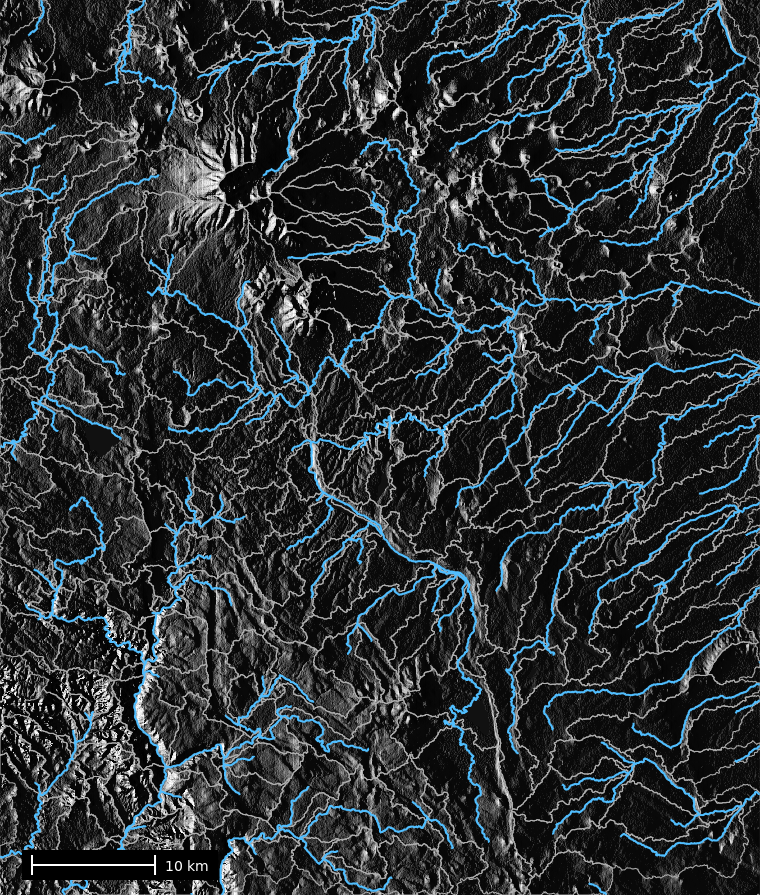
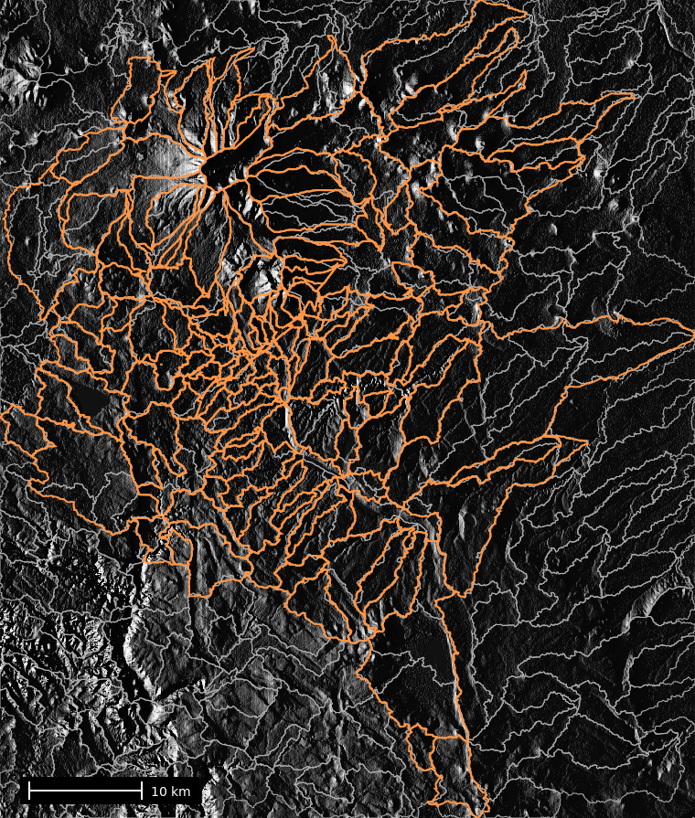
Gray lines are divides and blue lines are streams, drawn over a hillshade in
black with white highlights. The next sections look at how the tool produced
these and what controls how many there are.
## How the tool finds the divides
The four rasters are built in this order, and each one depends on the one
before it.
**Drainage direction.** For each cell, the neighbor it drains into.
**Accumulation.** For each cell, the number of cells that drain through it,
including itself. A cell on a ridge has a value of 1. A cell on a large river
can have a value in the hundreds of thousands. By default the tool splits each
cell's flow among its downhill neighbors, weighted by slope. This is called
multiple flow direction. The `-s` flag sends all flow to the single steepest
neighbor instead, which is the D8 method.
**Streams.** Cells whose accumulation is at or above the threshold.
**Basins.** The cells that drain into each stream segment. A basin has the
same id as its stream segment.
```{=html}
<figure class="plg-watershed">
<svg viewBox="0 0 420 250" role="img" aria-label="A three by three grid of cells with arrows pointing downhill and the count of cells draining through each">
<defs>
<marker id="plg-arrow" viewBox="0 0 10 10" refX="9" refY="5" markerWidth="6" markerHeight="6" orient="auto-start-reverse">
<path d="M 0 0 L 10 5 L 0 10 z" fill="#657e96"/>
</marker>
</defs>
<g stroke="#a76a3a" stroke-width="1.5">
<rect x="30" y="20" width="70" height="70" fill="#f0e3ce"/>
<rect x="100" y="20" width="70" height="70" fill="#f0e3ce"/>
<rect x="170" y="20" width="70" height="70" fill="#f0e3ce"/>
<rect x="30" y="90" width="70" height="70" fill="#f0e3ce"/>
<rect x="100" y="90" width="70" height="70" fill="#f0e3ce"/>
<rect x="170" y="90" width="70" height="70" fill="#f0e3ce"/>
<rect x="30" y="160" width="70" height="70" fill="#f0e3ce"/>
<rect x="100" y="160" width="70" height="70" fill="#d07944"/>
<rect x="170" y="160" width="70" height="70" fill="#f0e3ce"/>
</g>
<g stroke="#657e96" stroke-width="2.5" fill="none" marker-end="url(#plg-arrow)">
<line x1="72" y1="62" x2="108" y2="98"/>
<line x1="135" y1="66" x2="135" y2="104"/>
<line x1="198" y1="62" x2="162" y2="98"/>
<line x1="72" y1="132" x2="108" y2="168"/>
<line x1="135" y1="136" x2="135" y2="174"/>
<line x1="198" y1="132" x2="162" y2="168"/>
<line x1="88" y1="195" x2="112" y2="195"/>
<line x1="182" y1="195" x2="158" y2="195"/>
</g>
<g font-size="16" font-family="sans-serif" fill="#0a0a0a" font-weight="600">
<text x="40" y="40">1</text><text x="110" y="40">1</text><text x="180" y="40">1</text>
<text x="40" y="110">1</text><text x="110" y="110">4</text><text x="180" y="110">1</text>
<text x="40" y="180">1</text><text x="110" y="180" fill="#ffffff">9</text><text x="180" y="180">1</text>
</g>
<g font-size="13" font-family="sans-serif" fill="#4e4d4c">
<text x="265" y="45">arrow: drainage direction</text>
<text x="265" y="120">number: accumulation,</text>
<text x="265" y="138">cells draining through</text>
<text x="265" y="200">orange: the exit,</text>
<text x="265" y="218">all 9 cells pass here</text>
</g>
</svg>
<figcaption class="plg-caption">Each cell drains to a neighbor. The number in each cell is how many cells drain through it.</figcaption>
</figure>
```
## The threshold sets how many watersheds you get
The elevation data does not say where a stream begins, so the threshold is
used to decide. A low threshold treats small gullies as streams, each with its
own basin. A high threshold keeps only the larger channels, with fewer and
larger basins. The cell below runs the same DEM at two thresholds and counts
what comes out.
```{python}
# | label: threshold-sweep
from IPython.display import Markdown, display


def network_summary(threshold_km2, suffix):
    """Run r.watershed at one threshold and summarize what it produced."""
    threshold = round(threshold_km2 * 1e6 / cell_area_m2)
    tools.r_watershed(
        elevation="elevation@PERMANENT",
        threshold=threshold,
        stream=f"streams_{suffix}",
        basin=f"basins_{suffix}",
        overwrite=True,
    )
    stream_cells = int(tools.r_univar(map=f"streams_{suffix}", format="json")["n"])
    basin_count = len(tools.r_stats(input=f"basins_{suffix}", flags="n").text.split())
    area_km2 = n_cells * cell_area_m2 / 1e6
    # Channel length as cell count times cell size, ignoring diagonal steps.
    length_km = stream_cells * region["nsres"] / 1000
    return {
        "threshold km2": threshold_km2,
        "threshold cells": threshold,
        "basins": basin_count,
        "stream cells": stream_cells,
        "km of stream per km2": length_km / area_km2,
    }


def show_table(rows):
    """Render a list of dicts as a Markdown table."""
    header = list(rows[0])
    fmt = lambda v: f"{v:,.2f}" if isinstance(v, float) else f"{v:,}"
    lines = ["| " + " | ".join(header) + " |", "|" + "---:|" * len(header)]
    lines += ["| " + " | ".join(fmt(row[h]) for h in header) + " |" for row in rows]
    display(Markdown("\n".join(lines)))


show_table([network_summary(9.0, "9km2"), network_summary(0.45, "045km2")])
```
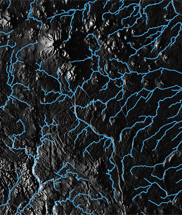
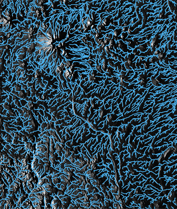
Between the two runs the number of watersheds differs by a factor of almost
twenty. Neither result is wrong. They describe the same terrain at different
levels of detail, and the threshold is what set that level.
```{python}
# | label: map-threshold
# | layout-ncol: 2
# | fig-cap: "The same DEM at two thresholds."
# | fig-subcap:
# | - "9 km2, 308 watersheds"
# | - "0.45 km2, 5,397 watersheds"
for suffix in ("9km2", "045km2"):
    tools.r_thin(input=f"streams_{suffix}", output=f"thin_{suffix}", overwrite=True)
    tools.r_to_vect(
        input=f"thin_{suffix}", output=f"vect_{suffix}", type="line", flags="v",
        overwrite=True,
    )

coarse = gj.Map(width=600, use_region=True)
coarse.d_rast(map="relief")
coarse.d_vect(map="vect_9km2", type="line", color=STREAM, width=2)
coarse.show()

fine = gj.Map(width=600, use_region=True)
fine.d_rast(map="relief")
fine.d_vect(map="vect_045km2", type="line", color=STREAM, width=2)
fine.show()
```
There is no single correct threshold. A reasonable choice depends on the
purpose. Common approaches are to match the drainage density of a mapped
stream network in similar terrain, to match channel heads observed in the
field, or to match the basin size that a later analysis expects. If the
threshold came from a tutorial, including this one, it is worth saying so in
your methods.
## The threshold is counted in cells
`r.watershed` takes the threshold as a number of cells. On this grid a cell is
900 square meters. If the same DEM is resampled to 90 m, a cell is 8,100
square meters, and the same cell count covers nine times the ground area.
Changing the cell size while keeping the cell count changes the result, even
though the threshold parameter looks the same.
```{python}
# | label: resolution
def run_at_resolution(res, suffix, threshold_cells=10000):
    """Run r.watershed on the DEM resampled to the given cell size."""
    dem = f"elevation_{suffix}"
    # RegionManager restores the original region when the block ends.
    with gs.RegionManager(raster="elevation@PERMANENT", res=res, flags="a"):
        reg = tools.g_region(flags="p", format="json")
        # Average the 30 m cells that fall inside each coarser cell. Reading
        # the 30 m raster directly at a coarser region would take one 30 m
        # cell per output cell instead, a nearest-neighbor resample.
        tools.r_resamp_stats(
            input="elevation@PERMANENT", output=dem, method="average", overwrite=True
        )
        tools.r_watershed(
            elevation=dem,
            threshold=threshold_cells,
            stream=f"streams_res{suffix}",
            basin=f"basins_res{suffix}",
            overwrite=True,
        )
        basins = len(tools.r_stats(input=f"basins_res{suffix}", flags="n").text.split())
        stream_cells = int(
            tools.r_univar(map=f"streams_res{suffix}", format="json")["n"]
        )
    return {
        "resolution m": int(reg["nsres"]),
        "cells in region": reg["rows"] * reg["cols"],
        "threshold cells": threshold_cells,
        "threshold km2": threshold_cells * reg["nsres"] * reg["ewres"] / 1e6,
        "basins": basins,
        "stream cells": stream_cells,
    }


# 30 m is the DEM's own cell size, so that run is unchanged by the resample.
show_table([run_at_resolution(30, "30"), run_at_resolution(90, "90")])
```
With the same 10,000 cell threshold, the 90 m run produces about fifteen
times fewer watersheds. This is why the main run set the threshold in square
kilometers and converted it to cells from the region. It also helps to record
the region settings alongside the threshold in your methods.
Two details in the code matter for a fair comparison. The coarser DEM is made
with `r.resamp.stats`, which averages the 30 m cells inside each 90 m cell.
Reading the 30 m raster at a 90 m region would instead pick one 30 m cell per
90 m cell, which keeps noise and drops detail. And the region change is wrapped
in `gs.RegionManager`, which puts the original region back when the block
ends, so later cells run on the 30 m grid without needing to reset it.
Cell size also limits what the DEM can represent. At 30 m, a 4 m wide swale
does not appear at all, and neither does the flow path through it. At 1 m, the
swale appears, but so do curbs, berms, and bridge decks, which the tool treats
as barriers. Stream length in particular depends on cell size and is hard to
compare across grids.
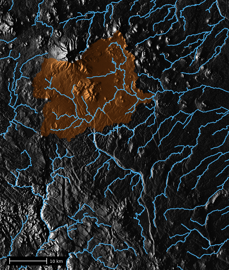
## The watershed above one point
Often the question is what drains to one place, such as a gauge, a culvert,
or an outfall. `r.water.outlet` follows the drainage raster upstream from a
coordinate and returns the watershed above it. The point needs to be on a
stream cell, so it is best taken from the computed stream network rather than
from a basemap. In this example the point is the cell with the largest
positive accumulation, which is the exit of the largest watershed that lies
entirely inside the region.
```{python}
# | label: outlet
tools.r_mapcalc(expression="accum_pos = if(accum > 0, accum, null())", overwrite=True)
cells = tools.r_stats(input="accum_pos", flags="gn").text
east, north, value = max(
    (line.split() for line in cells.strip().splitlines()),
    key=lambda parts: float(parts[2]),
)

tools.r_water_outlet(
    input="drainage", output="outlet_basin", coordinates=(east, north), overwrite=True
)

basin_cells = int(tools.r_univar(map="outlet_basin", format="json")["n"])
print(f"outlet: {east} E, {north} N")
print(f"accumulation at the outlet: {float(value):,.0f} cells "
      f"= {float(value) * cell_area_m2 / 1e6:.1f} km2")
print(f"r.water.outlet watershed:   {basin_cells:,} cells "
      f"= {basin_cells * cell_area_m2 / 1e6:.1f} km2")
```
The two areas agree to within a fraction of a percent. A small difference is
expected, because accumulation splits flow among neighbors while
`r.water.outlet` follows the single-direction drainage raster and counts whole
cells. A difference of tens of percent usually means the point is not on the
channel, often because the coordinate was picked from a basemap.
```{python}
# | label: map-outlet
# Tint the relief orange inside the watershed: copy the relief with the basin
# as a mask, then give the copy the same ramp ending in orange instead of
# white. MaskManager clears the mask when the block ends.
with gs.MaskManager(mask_name="outlet_basin"):
    tools.r_mapcalc(expression="outlet_shade = relief", overwrite=True)
rules = Path("outlet.rules")
rules.write_text(
    f"{shade['min']} 0:0:0\n{shade['median']} 70:35:10\n{shade['max']} 255:170:90\n"
)
tools.r_colors(map="outlet_shade", rules=str(rules))
rules.unlink()

outlet_map = gj.Map(width=760, use_region=True)
outlet_map.d_rast(map="relief")
outlet_map.d_rast(map="outlet_shade")
outlet_map.d_vect(map="streams_vect", type="line", color=STREAM, width=2)
outlet_map.d_barscale(**SCALE)
outlet_map.show()
```
## Watersheds cut by the region edge
The tool can only count cells inside the region. If a watershed extends past
the region edge, the cells outside are not counted, and `r.watershed` flags
this by making the accumulation negative. The absolute value is the count of
cells inside the region. The negative sign means the true value is larger by
an unknown amount.
The sign can be used to find which watersheds are affected.
```{python}
# | label: edge
tools.r_mapcalc(
    expression="edge_basins = if(accum < 0, basins, null())", overwrite=True
)
n_basins = len(tools.r_stats(input="basins", flags="n").text.split())
n_edge = len(tools.r_stats(input="edge_basins", flags="n").text.split())
neg = int(tools.r_univar(map="accum", format="json")["min"])

print(f"most negative accumulation: {neg:,} cells")
print(f"watersheds in the region:   {n_basins}")
print(f"cut by the region edge:     {n_edge}")
```
If the affected watersheds are the ones you need, the fix is to enlarge the
region so the whole contributing area is inside it, rerun, and clip the
results afterwards. For a headwater catchment the analysis extent may be close
to the site itself. For a site on a large river the extent can be many times
larger than the site. The `-a` flag makes all accumulation values positive,
which is convenient for display but does not change what was counted.
## Compare against the published watersheds
The Flagstaff dataset includes a `watersheds` vector from the City of
Flagstaff GIS. Overlaying it on the computed basins shows how a terrain-derived
delineation compares with a published one.
```{python}
# | label: map-compare
published = int(tools.v_info(map="watersheds@PERMANENT", format="json")["areas"])
print(f"published watersheds: {published}")
print(f"computed at {THRESHOLD_KM2} km2: {n_basins}")

compare = gj.Map(width=760, use_region=True)
compare.d_rast(map="relief")
compare.d_vect(map="basins_vect", fill_color="none", color=DIVIDE, width=1)
compare.d_vect(map="watersheds@PERMANENT", fill_color="none", color=CITY, width=2)
compare.d_barscale(**SCALE)
compare.show()
```
Orange is the city's map and gray is this run. The city's map covers only
part of the region, and its watersheds are smaller than those from a 9 km2
threshold, so several orange units often fall inside one gray one. Along the
major divides the two maps agree closely, since those follow the terrain. The
smaller boundaries differ, because the city drew them for stormwater
management at a scale that a single threshold does not reproduce. A
terrain-derived watershed is useful for understanding a published boundary,
but where a published boundary is required, that is the one to use.
## Bring your own DEM
The same workflow applies to any DEM. The difference is that you are
responsible for its vertical accuracy, its surface type, and its extent. The
cell below is not executed on this page. Run it against a GeoTIFF of your own.
```{python}
# | label: byo-data
# | eval: false
# 1) Create a project whose CRS comes from the tile itself.
project = Path.home() / "grassdata" / "my_watershed"
gs.create_project(project, filename="dem.tif")

# 2) Start a session and import, reprojecting if needed.
session = gj.init(project / "PERMANENT")
tools = Tools()
tools.r_import(input="dem.tif", output="dem", resample="bilinear")

# 3) Set the region from the imported map.
tools.g_region(raster="dem")

# 4) Fill NULL gaps, and only NULL gaps.
tools.r_fillnulls(input="dem", output="dem_nogaps", method="bilinear")

# 5) Route. Set the threshold in ground area and convert.
reg = tools.g_region(flags="p", format="json")
threshold = round(9.0 * 1e6 / (reg["nsres"] * reg["ewres"]))
tools.r_watershed(
    elevation="dem_nogaps",
    threshold=threshold,
    accumulation="accum",
    drainage="drainage",
    stream="streams",
    basin="basins",
)
```
::: {.callout-important}
## Fill the gaps, not the sinks
A NULL cell is missing data. `r.watershed` treats it as outside the region,
so a gap inside your area cuts off every flow path that reaches it. Fill gaps
with `r.fillnulls` before running the analysis.
A depression is a low spot with no outlet, which can be a real feature or
sensor noise. `r.watershed` does not need depressions filled, because it
routes flow through them with a least-cost search. Filling them beforehand
flattens real terrain and can produce artificial straight channels on the
flattened areas. If you know where real closed basins are, pass them with the
`depression=` option.
:::
Three things to check before using the result.
**Is the DEM a bare-earth model?** On a surface model that includes
vegetation, a wooded creek corridor can appear as a ridge, and the computed
channel may run beside the valley instead of through it. USGS 3DEP is bare
earth. Many photogrammetric and radar products are not.
**Is the extent large enough?** Check the negative accumulation cells. If they
reach the watersheds you need, the extent is too small.
**Is the terrain steep enough for the data?** A floodplain at a 0.02 percent
slope drops about 2 mm across a 10 m cell, while the vertical error of
national 10 m elevation data is on the order of a meter. On ground that flat,
the computed flow directions mostly reflect noise in the data. Channels that
wander or braid across a flat area are a sign of this, and a more accurate DEM
is usually the only fix.
## What r.watershed cannot tell you
The analysis uses only the shape of the terrain. It does not include
rainfall, soil, or time, so an accumulation value of 20,000 means 20,000 cells
and not a discharge. It does not know about culverts, storm drains, or
drainage tile, so computed flow can pile up behind road embankments that water
actually passes under. It is not a flood map. And a terrain-derived boundary
is not a substitute for the published one where a published one is required.
| If you need | Use instead |
|-------------|-------------|
| A stream network with topology and Strahler or Horton ordering | [`r.stream.extract`](https://grass.osgeo.org/grass-stable/manuals/r.stream.extract.html) and the `r.stream.*` addons |
| Overland flow with depth, time, or a rainfall event | [`r.sim.water`](https://grass.osgeo.org/grass-stable/manuals/r.sim.water.html) or a hydrodynamic model |
| Flow through culverts, storm drains, or tile | A pipe-network model, or a DEM you have burned the structures into by hand |
| A wetness index from a depressionless surface because a downstream model requires one | [`r.fill.dir`](https://grass.osgeo.org/grass-stable/manuals/r.fill.dir.html), or [`r.topidx`](https://grass.osgeo.org/grass-stable/manuals/r.topidx.html) |
| A boundary that matches a published one | The published dataset |
| Very large DEMs where speed matters more than accuracy on flat ground | [`r.terraflow`](https://grass.osgeo.org/grass-stable/manuals/r.terraflow.html) |
## Putting it together
1. A watershed is the area whose rain leaves through the same exit, and a divide is the boundary between two watersheds.
2. `r.watershed` links each cell to its downhill neighbor, counts the cells draining through each cell, marks cells above the threshold as streams, and groups cells by the stream segment they reach.
3. The threshold decides where a stream begins, and with it how many watersheds there are.
4. The threshold is counted in cells, so it is safer to set it in ground area, convert using the region, and record the region settings.
5. `r.water.outlet` returns the watershed above one point, and the point should come from the computed stream network.
6. Negative accumulation means a watershed extends past the region edge, and the fix is a larger region.
7. Fill NULL gaps before running the analysis, but do not fill depressions.
8. The result is a terrain-derived boundary. Compare it with the published one, and use the published one where it is required.
```{python}
# | label: cleanup
tools.g_remove(
    type="raster",
    name=(
        "streams_9km2,basins_9km2,streams_045km2,basins_045km2,"
        "thin_9km2,thin_045km2,streams_res30,basins_res30,"
        "streams_res90,basins_res90,elevation_30,elevation_90,accum_pos,"
        "edge_basins,outlet_shade"
    ),
    flags="f",
)
```
::: {.callout-tip}
## Try this without installing GRASS
OpenPlains runs GRASS tools like `r.watershed` in the browser, over an area you
draw on the map, with no local install. The platform is in beta.
[Request access](https://openplains.com/beta) to try it on your own
watershed.
:::
## References
Ehlschlaeger, C. (1989). Using the A^T search algorithm to develop hydrologic
models from digital elevation data. *Proceedings of the International Geographic
Information Systems (IGIS) Symposium '89*, 275-281. Baltimore, MD.
<http://chuck.ehlschlaeger.info/older/IGIS/paper.html>
Holmgren, P. (1994). Multiple flow direction algorithms for runoff modelling in
grid based elevation models: an empirical evaluation. *Hydrological Processes*,
8(4), 327-334. <https://doi.org/10.1002/hyp.3360080405>
Metz, M., Mitasova, H., & Harmon, R. S. (2011). Efficient extraction of drainage
networks from massive, radar-based elevation models with least cost path search.
*Hydrology and Earth System Sciences*, 15, 667-678.
<https://doi.org/10.5194/hess-15-667-2011>
White, C. T., Mitasova, H., Neteler, M., Petrasova, A., & Hofierka, J. (2026).
Geomorphometry in GRASS. In H. I. Reuter, C. H. Grohmann, & V. Lecours (Eds.),
*Geomorphometry: Concepts, software, applications* (2nd ed., Developments in
Soil Science, Vol. 37, pp. 417-442). Elsevier.
<https://doi.org/10.1016/B978-0-44-333376-7.00023-9>
GRASS Development Team. (2026). *Geographic Resources Analysis Support System
(GRASS) Software*. Open Source Geospatial Foundation.
<https://grass.osgeo.org>
When citing, include the method as well as the software. `r.watershed`
implements Ehlschlaeger's A^T least-cost search with the multiple flow
direction implementation by Metz and others.
## Data
The Flagstaff, Arizona sample dataset (`flagstaff_az_usa_epsg6341`, NAD83(2011)
/ UTM zone 12N, about 89 MB) was compiled by Michael Barton and Eunice
Villasenor at Arizona State University from USGS, NRCS, Coconino County, and
City of Flagstaff sources, with support from NSF grant 2303651. The `elevation`
map is a 30 m USGS DEM. The `watersheds` vector is from the City of Flagstaff
GIS. Credit the compilers and the originating agencies when you publish from
it. Download:
<https://grass.osgeo.org/sampledata/flagstaff_az_usa_epsg6341.zip>