STAC Tutorial – OpenPlains

Introduction

In this tutorial we will learn how to intergrate SpatioTemporal Asset Catalog (STAC) data into your GRASS workflow using the t.stac suite of tools for GRASS.

t.stac.catalog - is a tool for exploring SpatioTemporal Asset Catalogs metadata from a STAC API.
t.stac.collection - is a tool for exploring SpatioTemporal Asset Catalog (STAC) collection metadata.
t.stac.item - is a tool for exploring and importing SpatioTemporal Asset Catalog item metadata and assets into GRASS.

STAC is an open specification that provides a common structure for describing and cataloging geospatial information. STAC organizes earth observation data into a hierarchy of Catalogs → Collections → Items → Assets, making large archives of cloud-hosted imagery discoverable and accessible through a standard API. Major providers such as AWS, Google Cloud, and Microsoft Planetary Computer publish their datasets as STAC-compliant APIs, giving you a unified way to search and retrieve data across platforms.

The t.stac addon suite bridges these STAC APIs with GRASS’s spatio-temporal data management framework. Instead of manually browsing catalogs and downloading files, t.stac lets you:

Search by spatial extent and time window
Filter by metadata properties such as cloud cover, sun elevation, and resolution
Import matched assets directly into a GRASS project as a Space Time Raster Dataset (STRDS)

This tutorial walks through the full workflow: exploring a STAC catalog, querying Sentinel-2 imagery, downloading and importing it into GRASS, computing NDVI, and visualizing the time series.

The tutorial assumes you already have GRASS installed on your machine. If not please download and install GRASS before continuing the tutorial.

Getting Started

Start GRASS Session

# Import standard python packages
import sys
import subprocess
from IPython.display import display, JSON, HTML
import json
import pandas as pd
from pathlib import Path
import seaborn as sns
# import polars as pl

# Ask GRASS where its Python packages are and add them to the path
sys.path.append(
    subprocess.check_output(["grass", "--config", "python_path"], text=True).strip()
)

# Import the GRASS python packages we need
import grass.script as gs
import grass.jupyter as gj

Create a GRASS project

gs.create_project("stac", epsg="32119", overwrite=True)

and start a GRASS session.

session = gj.init("stac")

Install Addon

The t.stac addons require the following Python packages.

You can install them using pip or the Python package manager of your choice.

pip install pystac pystac_client tqdm

Now you can install the t.stac extensions.

gs.run_command("g.extension", extension="t.stac")

Define computational region

gs.run_command(
    "g.region", n=236687, s=210391, e=616042, w=598921, nsres=10, ewres=10, flags="pa"
)

projection: 99 (NAD83 / North Carolina)
zone:       0
datum:      nad83
ellipsoid:  grs80
north:      236690
south:      210390
west:       598920
east:       616050
nsres:      10
ewres:      10
rows:       2630
cols:       1713
cells:      4505190

STAC API

stac_url = "https://earth-search.aws.element84.com/v1/"

// renderValue is defined inside kvTable so OJS only sees one named cell,
// avoiding a circular reactive dependency between the two mutually recursive functions.
function kvTable(data) {
  function renderValue(v, key = "") {
    if (v === null)
      return htl.html`<span style="color:#999;font-style:italic">null</span>`;

    if (typeof v === "string") {
      const isImageUrl = /\.(jpg|jpeg|png|webp|gif)(\?.*)?$/i.test(v);
      const isCogUrl   = /\.tiff?(\?.*)?$/i.test(v);
      if (isImageUrl) {
        const img = htl.html`<img src="${v}" crossorigin="anonymous"
          style="max-width:260px;max-height:180px;border-radius:6px;object-fit:cover;display:block;margin-bottom:4px">`;
        img.onerror = () => img.style.display = "none";
        return htl.html`<div>${img}<a href="${v}" target="_blank"
          style="color:#1a73e8;font-size:11px;word-break:break-all">${v}</a></div>`;
      }
      if (isCogUrl)
        return htl.html`<div>
          <a href="${v}" target="_blank" style="color:#1a73e8;font-size:11px;word-break:break-all">${v}</a>
          ${cogMap(v)}
        </div>`;
      if (v.startsWith("http"))
        return htl.html`<a href="${v}" target="_blank"
          style="color:#1a73e8;word-break:break-all">${v}</a>`;
      return htl.html`<span style="color:#c41a16">${v}</span>`;
    }

    if (typeof v === "number")
      return htl.html`<span style="color:#1c00cf">${v}</span>`;

    if (typeof v === "boolean")
      return htl.html`<span style="color:#aa0d91">${String(v)}</span>`;

    if (Array.isArray(v)) {
      if (v.length === 0)
        return htl.html`<span style="color:#999">[ ]</span>`;
      if (v.every(i => typeof i !== "object") && v.length <= 8)
        return htl.html`<div style="display:flex;gap:4px;flex-wrap:wrap">
          ${v.map(i => htl.html`<span style="background:#e8f0fe;color:#1a73e8;
            font-size:11px;font-family:monospace;padding:2px 8px;border-radius:12px">${i}</span>`)}
        </div>`;
      return htl.html`<details>
        <summary style="cursor:pointer;color:#555;font-size:12px">[ ${v.length} items ]</summary>
        <ol style="margin:4px 0;padding-left:20px">
          ${v.map(i => htl.html`<li style="margin:2px 0">${renderValue(i)}</li>`)}
        </ol>
      </details>`;
    }

    if (typeof v === "object")
      return htl.html`<details>
        <summary style="cursor:pointer;color:#555;font-size:12px">{ ${Object.keys(v).length} keys }</summary>
        <div style="margin-top:4px">${kvTable(v)}</div>
      </details>`;

    return htl.html`<span>${String(v)}</span>`;
  }

  return htl.html`<table style="width:100%;border-collapse:collapse;font-size:13px">
    <thead>
      <tr>
        <th style="text-align:left;padding:8px 12px;background:#f5f5f5;color:#555;font-weight:600;width:35%">Property</th>
        <th style="text-align:left;padding:8px 12px;background:#f5f5f5;color:#555;font-weight:600">Value</th>
      </tr>
    </thead>
    <tbody>
      ${Object.entries(data).map(([k, v]) => htl.html`<tr style="border-bottom:1px solid #f0f0f0;vertical-align:top">
        <td style="padding:6px 12px;color:#881391;font-weight:600;font-family:monospace;font-size:12px">${k}</td>
        <td style="padding:6px 12px;font-family:monospace;font-size:12px">${renderValue(v, k)}</td>
      </tr>`)}
    </tbody>
  </table>`;
}

// cogMap renders a COG directly in the browser using georaster-layer-for-leaflet,
// which uses HTTP range requests to fetch only the needed overview tiles —
// no external tile server required. Bounds are read from the COG metadata.
function cogMap(url) {
  if (!document.querySelector("#leaflet-css")) {
    const link = document.createElement("link");
    link.id = "leaflet-css";
    link.rel = "stylesheet";
    link.href = "https://cdn.jsdelivr.net/npm/leaflet@1.9.4/dist/leaflet.css";
    document.head.appendChild(link);
  }

  // Inject a script once and poll until the global is available
  function loadScript(src, globalName) {
    return new Promise((resolve, reject) => {
      if (window[globalName]) { resolve(); return; }
      if (document.querySelector(`script[data-cogmap="${globalName}"]`)) {
        const poll = setInterval(() => {
          if (window[globalName]) { clearInterval(poll); resolve(); }
        }, 50);
        return;
      }
      const s = document.createElement("script");
      s.setAttribute("data-cogmap", globalName);
      s.src = src;
      s.onload = resolve;
      s.onerror = () => reject(new Error(`Failed to load ${globalName}`));
      document.head.appendChild(s);
    });
  }

  const el = htl.html`<details style="margin-top:8px">
    <summary style="cursor:pointer;color:#1a73e8;font-size:12px;padding:4px 0">🗺 View on map</summary>
    <div style="position:relative;height:300px;margin-top:8px;border-radius:6px;overflow:hidden;border:1px solid #e0e0e0">
      <div class="map-status" style="position:absolute;inset:0;display:flex;align-items:center;
        justify-content:center;background:#f9f9f9;color:#666;font-size:12px;font-family:monospace;z-index:1000">
        Loading...
      </div>
    </div>
  </details>`;

  let initialized = false;
  el.addEventListener("toggle", async () => {
    if (!el.open || initialized) return;
    initialized = true;
    const wrap   = el.querySelector("details > div");
    const status = el.querySelector(".map-status");
    try {
      await loadScript(
        "https://cdn.jsdelivr.net/npm/leaflet@1.9.4/dist/leaflet-src.js", "L");
      await loadScript(
        "https://cdn.jsdelivr.net/npm/georaster@1.6.2/dist/georaster.min.js", "parseGeoraster");
      await loadScript(
        "https://cdn.jsdelivr.net/npm/georaster-layer-for-leaflet@2.0.2/dist/georaster-layer-for-leaflet.min.js", "GeoRasterLayer");

      const { L, parseGeoraster, GeoRasterLayer } = window;
      const map = L.map(wrap, { scrollWheelZoom: false });
      L.tileLayer("https://{s}.tile.openstreetmap.org/{z}/{x}/{y}.png", {
        attribution: "© OpenStreetMap contributors", maxZoom: 19
      }).addTo(map);

      status.textContent = "Fetching COG...";
      const georaster = await parseGeoraster(url);

      const layer = new GeoRasterLayer({
        georaster,
        opacity: 0.85,
        resolution: 128,
        pixelValuesToColorFn: values => {
          const v = values[0];
          if (!v || v === georaster.noDataValue) return null;
          const t = Math.min(1, v / 3000);   // scale to 0-3000 (S2 L2A reflectance)
          const c = Math.round(t * 255);
          return `rgb(${c},${c},${c})`;
        }
      });
      layer.addTo(map);
      map.fitBounds(layer.getBounds());  // bounds come directly from COG metadata
      map.invalidateSize();
      status.remove();
    } catch (e) {
      status.textContent = `${e.message || "Failed to load COG"}`;
      status.style.color = "#c00";
    }
  });

  return el;
}

Searching STAC Catalogs

catalogs_json = gs.parse_command(
    "t.stac.catalog", url=stac_url, format="json"
)

df_catalogs = pd.json_normalize(catalogs_json)
df_catalogs.head()

Table 1

	type	id	stac_version	description	links	conformsTo	title
0	Catalog	earth-search-aws	1.1.0	A STAC API of public datasets on AWS	[{'rel': 'self', 'href': 'https://earth-search...	[https://api.stacspec.org/v1.0.0/core, https:/...	Earth Search by Element 84

Table 2

!t.stac.catalog url={stac_url} format=plain -b

Selected PROJ pipeline:
+proj=pipeline +step +inv +proj=lcc +lat_0=33.75 +lon_0=-79
+lat_1=36.1666666666667 +lat_2=34.3333333333333 +x_0=609601.22 +y_0=0
+no_defs +over +a=6378137 +rf=298.257222101 +towgs84=0.000,0.000,0.000
+step +proj=unitconvert +xy_in=rad +xy_out=deg
************************
---------------------------------------------------------------------------
Catalog: Earth Search by Element 84
---------------------------------------------------------------------------
Client Id: earth-search-aws
Client Description: A STAC API of public datasets on AWS
Client STAC Extensions: []
Client catalog_type: ABSOLUTE_PUBLISHED
---------------------------------------------------------------------------
Collections: 9
---------------------------------------------------------------------------
Collection Id | Collection Title
---------------------------------------------------------------------------
sentinel-2-pre-c1-l2a: Sentinel-2 Pre-Collection 1 Level-2A 
cop-dem-glo-30: Copernicus DEM GLO-30
naip: NAIP: National Agriculture Imagery Program
cop-dem-glo-90: Copernicus DEM GLO-90
landsat-c2-l2: Landsat Collection 2 Level-2
sentinel-2-l2a: Sentinel-2 Level-2A
sentinel-2-l1c: Sentinel-2 Level-1C
sentinel-2-c1-l2a: Sentinel-2 Collection 1 Level-2A
sentinel-1-grd: Sentinel-1 Level-1C Ground Range Detected (GRD)
---------------------------------------------------------------------------

Collection Metadata

items_json = gs.parse_command(
    "t.stac.item",
    url=stac_url,
    collection_id="sentinel-2-l2a",
    flags="m",
    format="json",
)

df_items = pd.json_normalize(items_json, max_level=0)
ojs_define(catalog_meta=df_items.drop(
    columns=["geometry", "links", "assets", "properties", "stac_extensions"],
    errors="ignore"
).to_dict(orient="records"))

Table 3

Table 4

!t.stac.item url={stac_url} collection_id="sentinel-2-l2a" format=plain -m

Selected PROJ pipeline:
+proj=pipeline +step +inv +proj=lcc +lat_0=33.75 +lon_0=-79
+lat_1=36.1666666666667 +lat_2=34.3333333333333 +x_0=609601.22 +y_0=0
+no_defs +over +a=6378137 +rf=298.257222101 +towgs84=0.000,0.000,0.000
+step +proj=unitconvert +xy_in=rad +xy_out=deg
************************
---------------------------------------------------------------------------

Collection Id: sentinel-2-l2a
Title: Sentinel-2 Level-2A
Description: Global Sentinel-2 data from the Multispectral Instrument (MSI) onboard Sentinel-2
bbox: [[-180, -90, 180, 90]]
Temporal Interval: [['2015-06-27T10:25:31.456000Z', None]]
License: proprietary
Keywords: ['sentinel', 'earth observation', 'esa']
Links: [{'rel': 'self', 'href': 'https://earth-search.aws.element84.com/v1/collections/sentinel-2-l2a', 'type': 'application/json'}, {'rel': 'cite-as', 'href': 'https://doi.org/10.5270/S2_-742ikth', 'title': 'Copernicus Sentinel-2 MSI Level-2A (L2A) Bottom-of-Atmosphere Radiance'}, {'rel': 'license', 'href': 'https://sentinel.esa.int/documents/247904/690755/Sentinel_Data_Legal_Notice', 'title': 'proprietary'}, {'rel': 'parent', 'href': 'https://earth-search.aws.element84.com/v1', 'type': 'application/json'}, {'rel': 'root', 'href': 'https://earth-search.aws.element84.com/v1/', 'type': 'application/json', 'title': 'Earth Search by Element 84'}, {'rel': 'items', 'href': 'https://earth-search.aws.element84.com/v1/collections/sentinel-2-l2a/items', 'type': 'application/geo+json'}, {'rel': 'http://www.opengis.net/def/rel/ogc/1.0/queryables', 'href': 'https://earth-search.aws.element84.com/v1/collections/sentinel-2-l2a/queryables', 'type': 'application/schema+json'}, {'rel': 'aggregate', 'href': 'https://earth-search.aws.element84.com/v1/collections/sentinel-2-l2a/aggregate', 'type': 'application/json', 'method': 'GET'}, {'rel': 'aggregations', 'href': 'https://earth-search.aws.element84.com/v1/collections/sentinel-2-l2a/aggregations', 'type': 'application/json'}]
Stac Extensions: ['https://stac-extensions.github.io/item-assets/v1.0.0/schema.json', 'https://stac-extensions.github.io/view/v1.0.0/schema.json', 'https://stac-extensions.github.io/scientific/v1.0.0/schema.json', 'https://stac-extensions.github.io/raster/v1.1.0/schema.json', 'https://stac-extensions.github.io/eo/v1.0.0/schema.json']

# Summaries:
---------------------------------------------------------------------------
    platform:
---------------------------------------------------------------------------
    constellation:
---------------------------------------------------------------------------
    instruments:
---------------------------------------------------------------------------
    gsd:
---------------------------------------------------------------------------
    view:off_nadir:
---------------------------------------------------------------------------
    sci:doi:
---------------------------------------------------------------------------
    eo:bands:
#         name: coastal
#         common_name: coastal
#         description: Coastal aerosol (band 1)
#         center_wavelength: 0.443
#         full_width_half_max: 0.027
#         name: blue
#         common_name: blue
#         description: Blue (band 2)
#         center_wavelength: 0.49
#         full_width_half_max: 0.098
#         name: green
#         common_name: green
#         description: Green (band 3)
#         center_wavelength: 0.56
#         full_width_half_max: 0.045
#         name: red
#         common_name: red
#         description: Red (band 4)
#         center_wavelength: 0.665
#         full_width_half_max: 0.038
#         name: rededge1
#         common_name: rededge
#         description: Red edge 1 (band 5)
#         center_wavelength: 0.704
#         full_width_half_max: 0.019
#         name: rededge2
#         common_name: rededge
#         description: Red edge 2 (band 6)
#         center_wavelength: 0.74
#         full_width_half_max: 0.018
#         name: rededge3
#         common_name: rededge
#         description: Red edge 3 (band 7)
#         center_wavelength: 0.783
#         full_width_half_max: 0.028
#         name: nir
#         common_name: nir
#         description: NIR 1 (band 8)
#         center_wavelength: 0.842
#         full_width_half_max: 0.145
#         name: nir08
#         common_name: nir08
#         description: NIR 2 (band 8A)
#         center_wavelength: 0.865
#         full_width_half_max: 0.033
#         name: nir09
#         common_name: nir09
#         description: NIR 3 (band 9)
#         center_wavelength: 0.945
#         full_width_half_max: 0.026
#         name: cirrus
#         common_name: cirrus
#         description: Cirrus (band 10)
#         center_wavelength: 1.3735
#         full_width_half_max: 0.075
#         name: swir16
#         common_name: swir16
#         description: SWIR 1 (band 11)
#         center_wavelength: 1.61
#         full_width_half_max: 0.143
#         name: swir22
#         common_name: swir22
#         description: SWIR 2 (band 12)
#         center_wavelength: 2.19
#         full_width_half_max: 0.242

# Extra Fields:
# Extra Fields not found.
---------------------------------------------------------------------------

Inputs.table(catalog_meta, {width: "100%"})

Query Items by datetime and display table

items_json = gs.parse_command(
    "t.stac.item",
    url=stac_url,
    collection_id="sentinel-2-l2a",
    flags="i",
    datetime="2024-04-01/2024-09-30",
    format="json",
)
num_items = len(df_items)
df_items = pd.json_normalize(items_json, max_level=0)
ojs_define(items_table=df_items.drop(
    columns=["geometry", "links", "assets", "properties", "stac_extensions", "type"],
    errors="ignore"
).head(10).to_dict(orient="records"))

Table 5

Table 6

!t.stac.item url={stac_url} collection_id="sentinel-2-l2a" datetime="2024-04-01/2024-09-30" format=plain -i

Selected PROJ pipeline:
+proj=pipeline +step +inv +proj=lcc +lat_0=33.75 +lon_0=-79
+lat_1=36.1666666666667 +lat_2=34.3333333333333 +x_0=609601.22 +y_0=0
+no_defs +over +a=6378137 +rf=298.257222101 +towgs84=0.000,0.000,0.000
+step +proj=unitconvert +xy_in=rad +xy_out=deg
************************
Search Matched: 38 items
bbox: [-79.11829907, 35.64652526, -78.92857699, 35.88363678]
Items Found: 38
Collection ID: sentinel-2-l2a
Item: S2A_17SPV_20240929_0_L2A
Geometry: {'type': 'Polygon', 'coordinates': [[[-79.88850843890832, 36.1397316133374], [-79.9021350633042, 35.14992495410683], [-78.69735281151316, 35.13301555004904], [-78.66879673080497, 36.12219793572046], [-79.88850843890832, 36.1397316133374]]]}
Bbox: [-79.9021350633042, 35.13301555004904, -78.66879673080497, 36.1397316133374]
Datetime: 2024-09-29 16:13:28.352000+00:00
Start Datetime not found.
End Datetime not found.
Extra Fields:
---------------------------------------------------------------------------
Extensions:
---------------------------------------------------------------------------
    https://stac-extensions.github.io/processing/v1.1.0/schema.json
    https://stac-extensions.github.io/projection/v2.0.0/schema.json
    https://stac-extensions.github.io/raster/v1.1.0/schema.json
    https://stac-extensions.github.io/mgrs/v1.0.0/schema.json
    https://stac-extensions.github.io/grid/v1.1.0/schema.json
    https://stac-extensions.github.io/eo/v1.1.0/schema.json
    https://stac-extensions.github.io/view/v1.0.0/schema.json
---------------------------------------------------------------------------
Properties:
#     created: 2024-09-29T23:18:47.401Z
#     platform: sentinel-2a
#     constellation: sentinel-2
---------------------------------------------------------------------------
    instruments:
#     eo:cloud_cover: 74.087
#     mgrs:utm_zone: 17
#     mgrs:latitude_band: S
#     mgrs:grid_square: PV
#     grid:code: MGRS-17SPV
#     view:sun_azimuth: 159.030812026265
#     view:sun_elevation: 49.5733673337649
#     s2:degraded_msi_data_percentage: 0.0133
#     s2:nodata_pixel_percentage: 0
#     s2:saturated_defective_pixel_percentage: 0
#     s2:cloud_shadow_percentage: 1.035474
#     s2:vegetation_percentage: 17.151682
#     s2:not_vegetated_percentage: 2.54457
#     s2:water_percentage: 0.531116
#     s2:unclassified_percentage: 4.430241
#     s2:medium_proba_clouds_percentage: 14.835113
#     s2:high_proba_clouds_percentage: 59.251028
#     s2:thin_cirrus_percentage: 0.000859
#     s2:snow_ice_percentage: 0
#     s2:product_type: S2MSI2A
#     s2:processing_baseline: 05.11
#     s2:product_uri: S2A_MSIL2A_20240929T160051_N0511_R097_T17SPV_20240929T214148.SAFE
#     s2:generation_time: 2024-09-29T21:41:48.000000Z
#     s2:datatake_id: GS2A_20240929T160051_048428_N05.11
#     s2:datatake_type: INS-NOBS
#     s2:datastrip_id: S2A_OPER_MSI_L2A_DS_2APS_20240929T214148_S20240929T160935_N05.11
#     s2:granule_id: S2A_OPER_MSI_L2A_TL_2APS_20240929T214148_A048428_T17SPV_N05.11
#     s2:reflectance_conversion_factor: 0.99535952936181
#     datetime: 2024-09-29T16:13:28.352000Z
#     s2:sequence: 0
#     earthsearch:s3_path: s3://sentinel-cogs/sentinel-s2-l2a-cogs/17/S/PV/2024/9/S2A_17SPV_20240929_0_L2A
#     earthsearch:payload_id: roda-sentinel2/workflow-sentinel2-to-stac/4358322d6f3b7cc6a1345f1e4582a193
#     earthsearch:boa_offset_applied: True
---------------------------------------------------------------------------

     processing:software:
#         sentinel2-to-stac: 0.1.1
#     processing:software: {'sentinel2-to-stac': '0.1.1'}
#     updated: 2024-09-29T23:18:47.401Z
#     proj:code: EPSG:32617
Collection ID: sentinel-2-l2a
Item: S2B_17SPV_20240924_0_L2A
Geometry: {'type': 'Polygon', 'coordinates': [[[-79.88850843890832, 36.1397316133374], [-79.9021350633042, 35.14992495410683], [-78.69735281151316, 35.13301555004904], [-78.66879673080497, 36.12219793572046], [-79.88850843890832, 36.1397316133374]]]}
Bbox: [-79.9021350633042, 35.13301555004904, -78.66879673080497, 36.1397316133374]
Datetime: 2024-09-24 16:13:24.693000+00:00
Start Datetime not found.
End Datetime not found.
Extra Fields:
---------------------------------------------------------------------------
Extensions:
---------------------------------------------------------------------------
    https://stac-extensions.github.io/eo/v1.1.0/schema.json
    https://stac-extensions.github.io/grid/v1.1.0/schema.json
    https://stac-extensions.github.io/processing/v1.1.0/schema.json
    https://stac-extensions.github.io/raster/v1.1.0/schema.json
    https://stac-extensions.github.io/view/v1.0.0/schema.json
    https://stac-extensions.github.io/projection/v2.0.0/schema.json
    https://stac-extensions.github.io/mgrs/v1.0.0/schema.json
---------------------------------------------------------------------------
Properties:
#     created: 2024-09-25T06:45:08.923Z
#     platform: sentinel-2b
#     constellation: sentinel-2
---------------------------------------------------------------------------
    instruments:
#     eo:cloud_cover: 99.348462
#     mgrs:utm_zone: 17
#     mgrs:latitude_band: S
#     mgrs:grid_square: PV
#     grid:code: MGRS-17SPV
#     view:sun_azimuth: 157.455076519409
#     view:sun_elevation: 51.2968775702621
#     s2:degraded_msi_data_percentage: 0.0052
#     s2:nodata_pixel_percentage: 0
#     s2:saturated_defective_pixel_percentage: 0
#     s2:cloud_shadow_percentage: 0.600874
#     s2:vegetation_percentage: 0.012064
#     s2:not_vegetated_percentage: 0.00723
#     s2:water_percentage: 0.001035
#     s2:unclassified_percentage: 0.030182
#     s2:medium_proba_clouds_percentage: 1.05707
#     s2:high_proba_clouds_percentage: 98.291391
#     s2:thin_cirrus_percentage: 0
#     s2:snow_ice_percentage: 0
#     s2:product_type: S2MSI2A
#     s2:processing_baseline: 05.11
#     s2:product_uri: S2B_MSIL2A_20240924T155909_N0511_R097_T17SPV_20240924T215647.SAFE
#     s2:generation_time: 2024-09-24T21:56:47.000000Z
#     s2:datatake_id: GS2B_20240924T155909_039448_N05.11
#     s2:datatake_type: INS-NOBS
#     s2:datastrip_id: S2B_OPER_MSI_L2A_DS_2BPS_20240924T215647_S20240924T161235_N05.11
#     s2:granule_id: S2B_OPER_MSI_L2A_TL_2BPS_20240924T215647_A039448_T17SPV_N05.11
#     s2:reflectance_conversion_factor: 0.992555642055685
#     datetime: 2024-09-24T16:13:24.693000Z
#     s2:sequence: 0
#     earthsearch:s3_path: s3://sentinel-cogs/sentinel-s2-l2a-cogs/17/S/PV/2024/9/S2B_17SPV_20240924_0_L2A
#     earthsearch:payload_id: roda-sentinel2/workflow-sentinel2-to-stac/5da8ad2203ff3aeeb1380ac4891c6811
#     earthsearch:boa_offset_applied: True
---------------------------------------------------------------------------

     processing:software:
#         sentinel2-to-stac: 0.1.1
#     processing:software: {'sentinel2-to-stac': '0.1.1'}
#     updated: 2024-09-25T06:45:08.923Z
#     proj:code: EPSG:32617
Collection ID: sentinel-2-l2a
Item: S2A_17SPV_20240919_0_L2A
Geometry: {'type': 'Polygon', 'coordinates': [[[-79.88850843890832, 36.1397316133374], [-79.9021350633042, 35.14992495410683], [-78.69735281151316, 35.13301555004904], [-78.66879673080497, 36.12219793572046], [-79.88850843890832, 36.1397316133374]]]}
Bbox: [-79.9021350633042, 35.13301555004904, -78.66879673080497, 36.1397316133374]
Datetime: 2024-09-19 16:13:27.093000+00:00
Start Datetime not found.
End Datetime not found.
Extra Fields:
---------------------------------------------------------------------------
Extensions:
---------------------------------------------------------------------------
    https://stac-extensions.github.io/view/v1.0.0/schema.json
    https://stac-extensions.github.io/processing/v1.1.0/schema.json
    https://stac-extensions.github.io/mgrs/v1.0.0/schema.json
    https://stac-extensions.github.io/eo/v1.1.0/schema.json
    https://stac-extensions.github.io/grid/v1.1.0/schema.json
    https://stac-extensions.github.io/raster/v1.1.0/schema.json
    https://stac-extensions.github.io/projection/v2.0.0/schema.json
---------------------------------------------------------------------------
Properties:
#     created: 2024-09-20T01:57:52.703Z
#     platform: sentinel-2a
#     constellation: sentinel-2
---------------------------------------------------------------------------
    instruments:
#     eo:cloud_cover: 72.722346
#     mgrs:utm_zone: 17
#     mgrs:latitude_band: S
#     mgrs:grid_square: PV
#     grid:code: MGRS-17SPV
#     view:sun_azimuth: 155.767671819208
#     view:sun_elevation: 52.9984536527629
#     s2:degraded_msi_data_percentage: 0.0622
#     s2:nodata_pixel_percentage: 0
#     s2:saturated_defective_pixel_percentage: 0
#     s2:cloud_shadow_percentage: 2.901951
#     s2:vegetation_percentage: 17.622864
#     s2:not_vegetated_percentage: 2.652742
#     s2:water_percentage: 0.198822
#     s2:unclassified_percentage: 3.66454
#     s2:medium_proba_clouds_percentage: 19.171326
#     s2:high_proba_clouds_percentage: 53.275347
#     s2:thin_cirrus_percentage: 0.275673
#     s2:snow_ice_percentage: 0
#     s2:product_type: S2MSI2A
#     s2:processing_baseline: 05.11
#     s2:product_uri: S2A_MSIL2A_20240919T155931_N0511_R097_T17SPV_20240919T235348.SAFE
#     s2:generation_time: 2024-09-19T23:53:48.000000Z
#     s2:datatake_id: GS2A_20240919T155931_048285_N05.11
#     s2:datatake_type: INS-NOBS
#     s2:datastrip_id: S2A_OPER_MSI_L2A_DS_2APS_20240919T235348_S20240919T160354_N05.11
#     s2:granule_id: S2A_OPER_MSI_L2A_TL_2APS_20240919T235348_A048285_T17SPV_N05.11
#     s2:reflectance_conversion_factor: 0.989818874139801
#     datetime: 2024-09-19T16:13:27.093000Z
#     s2:sequence: 0
#     earthsearch:s3_path: s3://sentinel-cogs/sentinel-s2-l2a-cogs/17/S/PV/2024/9/S2A_17SPV_20240919_0_L2A
#     earthsearch:payload_id: roda-sentinel2/workflow-sentinel2-to-stac/15f081a7f9bdd87cc5f4cabfb05f981d
#     earthsearch:boa_offset_applied: True
---------------------------------------------------------------------------

     processing:software:
#         sentinel2-to-stac: 0.1.1
#     processing:software: {'sentinel2-to-stac': '0.1.1'}
#     updated: 2024-09-20T01:57:52.703Z
#     proj:code: EPSG:32617
Collection ID: sentinel-2-l2a
Item: S2B_17SPV_20240914_0_L2A
Geometry: {'type': 'Polygon', 'coordinates': [[[-79.88850843890832, 36.1397316133374], [-79.9021350633042, 35.14992495410683], [-78.69735281151316, 35.13301555004904], [-78.66879673080497, 36.12219793572046], [-79.88850843890832, 36.1397316133374]]]}
Bbox: [-79.9021350633042, 35.13301555004904, -78.66879673080497, 36.1397316133374]
Datetime: 2024-09-14 16:13:25.669000+00:00
Start Datetime not found.
End Datetime not found.
Extra Fields:
---------------------------------------------------------------------------
Extensions:
---------------------------------------------------------------------------
    https://stac-extensions.github.io/grid/v1.1.0/schema.json
    https://stac-extensions.github.io/view/v1.0.0/schema.json
    https://stac-extensions.github.io/processing/v1.1.0/schema.json
    https://stac-extensions.github.io/eo/v1.1.0/schema.json
    https://stac-extensions.github.io/projection/v2.0.0/schema.json
    https://stac-extensions.github.io/mgrs/v1.0.0/schema.json
    https://stac-extensions.github.io/raster/v1.1.0/schema.json
---------------------------------------------------------------------------
Properties:
#     created: 2024-09-15T00:07:17.726Z
#     platform: sentinel-2b
#     constellation: sentinel-2
---------------------------------------------------------------------------
    instruments:
#     eo:cloud_cover: 79.828173
#     mgrs:utm_zone: 17
#     mgrs:latitude_band: S
#     mgrs:grid_square: PV
#     grid:code: MGRS-17SPV
#     view:sun_azimuth: 153.914058363041
#     view:sun_elevation: 54.654514165176
#     s2:degraded_msi_data_percentage: 0.007
#     s2:nodata_pixel_percentage: 0
#     s2:saturated_defective_pixel_percentage: 0
#     s2:cloud_shadow_percentage: 3.506305
#     s2:vegetation_percentage: 15.025803
#     s2:not_vegetated_percentage: 0.845717
#     s2:water_percentage: 0.04352
#     s2:unclassified_percentage: 0.7308
#     s2:medium_proba_clouds_percentage: 25.53083
#     s2:high_proba_clouds_percentage: 41.27472
#     s2:thin_cirrus_percentage: 13.022627
#     s2:snow_ice_percentage: 0
#     s2:product_type: S2MSI2A
#     s2:processing_baseline: 05.11
#     s2:product_uri: S2B_MSIL2A_20240914T155819_N0511_R097_T17SPV_20240914T213957.SAFE
#     s2:generation_time: 2024-09-14T21:39:57.000000Z
#     s2:datatake_id: GS2B_20240914T155819_039305_N05.11
#     s2:datatake_type: INS-NOBS
#     s2:datastrip_id: S2B_OPER_MSI_L2A_DS_2BPS_20240914T213957_S20240914T160632_N05.11
#     s2:granule_id: S2B_OPER_MSI_L2A_TL_2BPS_20240914T213957_A039305_T17SPV_N05.11
#     s2:reflectance_conversion_factor: 0.987167209559927
#     datetime: 2024-09-14T16:13:25.669000Z
#     s2:sequence: 0
#     earthsearch:s3_path: s3://sentinel-cogs/sentinel-s2-l2a-cogs/17/S/PV/2024/9/S2B_17SPV_20240914_0_L2A
#     earthsearch:payload_id: roda-sentinel2/workflow-sentinel2-to-stac/f6a2326175b22d8a18f9cfdcf10d61a6
#     earthsearch:boa_offset_applied: True
---------------------------------------------------------------------------

     processing:software:
#         sentinel2-to-stac: 0.1.1
#     processing:software: {'sentinel2-to-stac': '0.1.1'}
#     updated: 2024-09-15T00:07:17.726Z
#     proj:code: EPSG:32617
Collection ID: sentinel-2-l2a
Item: S2A_17SPV_20240909_0_L2A
Geometry: {'type': 'Polygon', 'coordinates': [[[-79.88850843890832, 36.1397316133374], [-79.9021350633042, 35.14992495410683], [-78.69735281151316, 35.13301555004904], [-78.66879673080497, 36.12219793572046], [-79.88850843890832, 36.1397316133374]]]}
Bbox: [-79.9021350633042, 35.13301555004904, -78.66879673080497, 36.1397316133374]
Datetime: 2024-09-09 16:13:25.358000+00:00
Start Datetime not found.
End Datetime not found.
Extra Fields:
---------------------------------------------------------------------------
Extensions:
---------------------------------------------------------------------------
    https://stac-extensions.github.io/grid/v1.1.0/schema.json
    https://stac-extensions.github.io/mgrs/v1.0.0/schema.json
    https://stac-extensions.github.io/projection/v2.0.0/schema.json
    https://stac-extensions.github.io/eo/v1.1.0/schema.json
    https://stac-extensions.github.io/view/v1.0.0/schema.json
    https://stac-extensions.github.io/raster/v1.1.0/schema.json
    https://stac-extensions.github.io/processing/v1.1.0/schema.json
---------------------------------------------------------------------------
Properties:
#     created: 2024-09-10T01:00:11.150Z
#     platform: sentinel-2a
#     constellation: sentinel-2
---------------------------------------------------------------------------
    instruments:
#     eo:cloud_cover: 0.583943
#     mgrs:utm_zone: 17
#     mgrs:latitude_band: S
#     mgrs:grid_square: PV
#     grid:code: MGRS-17SPV
#     view:sun_azimuth: 151.939335784169
#     view:sun_elevation: 56.2633790627923
#     s2:degraded_msi_data_percentage: 0.0076
#     s2:nodata_pixel_percentage: 0
#     s2:saturated_defective_pixel_percentage: 0
#     s2:cloud_shadow_percentage: 0.282156
#     s2:vegetation_percentage: 90.927249
#     s2:not_vegetated_percentage: 5.989857
#     s2:water_percentage: 1.08207
#     s2:unclassified_percentage: 0.802021
#     s2:medium_proba_clouds_percentage: 0.458496
#     s2:high_proba_clouds_percentage: 0.11125
#     s2:thin_cirrus_percentage: 0.014197
#     s2:snow_ice_percentage: 0
#     s2:product_type: S2MSI2A
#     s2:processing_baseline: 05.11
#     s2:product_uri: S2A_MSIL2A_20240909T155901_N0511_R097_T17SPV_20240909T230449.SAFE
#     s2:generation_time: 2024-09-09T23:04:49.000000Z
#     s2:datatake_id: GS2A_20240909T155901_048142_N05.11
#     s2:datatake_type: INS-NOBS
#     s2:datastrip_id: S2A_OPER_MSI_L2A_DS_2APS_20240909T230449_S20240909T161131_N05.11
#     s2:granule_id: S2A_OPER_MSI_L2A_TL_2APS_20240909T230449_A048142_T17SPV_N05.11
#     s2:reflectance_conversion_factor: 0.984620442079431
#     datetime: 2024-09-09T16:13:25.358000Z
#     s2:sequence: 0
#     earthsearch:s3_path: s3://sentinel-cogs/sentinel-s2-l2a-cogs/17/S/PV/2024/9/S2A_17SPV_20240909_0_L2A
#     earthsearch:payload_id: roda-sentinel2/workflow-sentinel2-to-stac/4d9c572c80f8d121e13f58841e96ab3f
#     earthsearch:boa_offset_applied: True
---------------------------------------------------------------------------

     processing:software:
#         sentinel2-to-stac: 0.1.1
#     processing:software: {'sentinel2-to-stac': '0.1.1'}
#     updated: 2024-09-10T01:00:11.150Z
#     proj:code: EPSG:32617
Collection ID: sentinel-2-l2a
Item: S2B_17SPV_20240904_0_L2A
Geometry: {'type': 'Polygon', 'coordinates': [[[-79.88850843890832, 36.1397316133374], [-79.9021350633042, 35.14992495410683], [-78.69735281151316, 35.13301555004904], [-78.66879673080497, 36.12219793572046], [-79.88850843890832, 36.1397316133374]]]}
Bbox: [-79.9021350633042, 35.13301555004904, -78.66879673080497, 36.1397316133374]
Datetime: 2024-09-04 16:13:28.898000+00:00
Start Datetime not found.
End Datetime not found.
Extra Fields:
---------------------------------------------------------------------------
Extensions:
---------------------------------------------------------------------------
    https://stac-extensions.github.io/view/v1.0.0/schema.json
    https://stac-extensions.github.io/grid/v1.1.0/schema.json
    https://stac-extensions.github.io/processing/v1.1.0/schema.json
    https://stac-extensions.github.io/mgrs/v1.0.0/schema.json
    https://stac-extensions.github.io/projection/v2.0.0/schema.json
    https://stac-extensions.github.io/raster/v1.1.0/schema.json
    https://stac-extensions.github.io/eo/v1.1.0/schema.json
---------------------------------------------------------------------------
Properties:
#     created: 2024-09-04T23:56:25.240Z
#     platform: sentinel-2b
#     constellation: sentinel-2
---------------------------------------------------------------------------
    instruments:
#     eo:cloud_cover: 85.910875
#     mgrs:utm_zone: 17
#     mgrs:latitude_band: S
#     mgrs:grid_square: PV
#     grid:code: MGRS-17SPV
#     view:sun_azimuth: 149.877490350857
#     view:sun_elevation: 57.820905383914
#     s2:degraded_msi_data_percentage: 0.0027
#     s2:nodata_pixel_percentage: 0
#     s2:saturated_defective_pixel_percentage: 0
#     s2:cloud_shadow_percentage: 0.144353
#     s2:vegetation_percentage: 11.959764
#     s2:not_vegetated_percentage: 0.834155
#     s2:water_percentage: 0.120812
#     s2:unclassified_percentage: 1.003573
#     s2:medium_proba_clouds_percentage: 31.174442
#     s2:high_proba_clouds_percentage: 35.781747
#     s2:thin_cirrus_percentage: 18.954691
#     s2:snow_ice_percentage: 0
#     s2:product_type: S2MSI2A
#     s2:processing_baseline: 05.11
#     s2:product_uri: S2B_MSIL2A_20240904T155819_N0511_R097_T17SPV_20240904T214205.SAFE
#     s2:generation_time: 2024-09-04T21:42:05.000000Z
#     s2:datatake_id: GS2B_20240904T155819_039162_N05.11
#     s2:datatake_type: INS-NOBS
#     s2:datastrip_id: S2B_OPER_MSI_L2A_DS_2BPS_20240904T214205_S20240904T160310_N05.11
#     s2:granule_id: S2B_OPER_MSI_L2A_TL_2BPS_20240904T214205_A039162_T17SPV_N05.11
#     s2:reflectance_conversion_factor: 0.982194975113435
#     datetime: 2024-09-04T16:13:28.898000Z
#     s2:sequence: 0
#     earthsearch:s3_path: s3://sentinel-cogs/sentinel-s2-l2a-cogs/17/S/PV/2024/9/S2B_17SPV_20240904_0_L2A
#     earthsearch:payload_id: roda-sentinel2/workflow-sentinel2-to-stac/a34722af06ac7f7dc3a6579ff0c804bc
#     earthsearch:boa_offset_applied: True
---------------------------------------------------------------------------

     processing:software:
#         sentinel2-to-stac: 0.1.1
#     processing:software: {'sentinel2-to-stac': '0.1.1'}
#     updated: 2024-09-04T23:56:25.240Z
#     proj:code: EPSG:32617
Collection ID: sentinel-2-l2a
Item: S2A_17SPV_20240830_0_L2A
Geometry: {'type': 'Polygon', 'coordinates': [[[-79.88850843890832, 36.1397316133374], [-79.9021350633042, 35.14992495410683], [-78.69735281151316, 35.13301555004904], [-78.66879673080497, 36.12219793572046], [-79.88850843890832, 36.1397316133374]]]}
Bbox: [-79.9021350633042, 35.13301555004904, -78.66879673080497, 36.1397316133374]
Datetime: 2024-08-30 16:13:25.079000+00:00
Start Datetime not found.
End Datetime not found.
Extra Fields:
---------------------------------------------------------------------------
Extensions:
---------------------------------------------------------------------------
    https://stac-extensions.github.io/mgrs/v1.0.0/schema.json
    https://stac-extensions.github.io/processing/v1.1.0/schema.json
    https://stac-extensions.github.io/projection/v2.0.0/schema.json
    https://stac-extensions.github.io/raster/v1.1.0/schema.json
    https://stac-extensions.github.io/view/v1.0.0/schema.json
    https://stac-extensions.github.io/grid/v1.1.0/schema.json
    https://stac-extensions.github.io/eo/v1.1.0/schema.json
---------------------------------------------------------------------------
Properties:
#     created: 2024-08-31T00:58:00.459Z
#     platform: sentinel-2a
#     constellation: sentinel-2
---------------------------------------------------------------------------
    instruments:
#     eo:cloud_cover: 29.260489
#     mgrs:utm_zone: 17
#     mgrs:latitude_band: S
#     mgrs:grid_square: PV
#     grid:code: MGRS-17SPV
#     view:sun_azimuth: 147.666056006198
#     view:sun_elevation: 59.2994603957414
#     s2:degraded_msi_data_percentage: 0.0075
#     s2:nodata_pixel_percentage: 0
#     s2:saturated_defective_pixel_percentage: 0
#     s2:cloud_shadow_percentage: 2.806995
#     s2:vegetation_percentage: 60.253859
#     s2:not_vegetated_percentage: 4.589577
#     s2:water_percentage: 0.798839
#     s2:unclassified_percentage: 2.123901
#     s2:medium_proba_clouds_percentage: 8.565114
#     s2:high_proba_clouds_percentage: 7.006772
#     s2:thin_cirrus_percentage: 13.688605
#     s2:snow_ice_percentage: 0
#     s2:product_type: S2MSI2A
#     s2:processing_baseline: 05.11
#     s2:product_uri: S2A_MSIL2A_20240830T155901_N0511_R097_T17SPV_20240830T230248.SAFE
#     s2:generation_time: 2024-08-30T23:02:48.000000Z
#     s2:datatake_id: GS2A_20240830T155901_047999_N05.11
#     s2:datatake_type: INS-NOBS
#     s2:datastrip_id: S2A_OPER_MSI_L2A_DS_2APS_20240830T230248_S20240830T161243_N05.11
#     s2:granule_id: S2A_OPER_MSI_L2A_TL_2APS_20240830T230248_A047999_T17SPV_N05.11
#     s2:reflectance_conversion_factor: 0.979908290720517
#     datetime: 2024-08-30T16:13:25.079000Z
#     s2:sequence: 0
#     earthsearch:s3_path: s3://sentinel-cogs/sentinel-s2-l2a-cogs/17/S/PV/2024/8/S2A_17SPV_20240830_0_L2A
#     earthsearch:payload_id: roda-sentinel2/workflow-sentinel2-to-stac/f5abdfe94133d858b559236189785d38
#     earthsearch:boa_offset_applied: True
---------------------------------------------------------------------------

     processing:software:
#         sentinel2-to-stac: 0.1.1
#     processing:software: {'sentinel2-to-stac': '0.1.1'}
#     updated: 2024-08-31T00:58:00.459Z
#     proj:code: EPSG:32617
Collection ID: sentinel-2-l2a
Item: S2B_17SPV_20240825_0_L2A
Geometry: {'type': 'Polygon', 'coordinates': [[[-79.88850843890832, 36.1397316133374], [-79.9021350633042, 35.14992495410683], [-78.69735281151316, 35.13301555004904], [-78.66879673080497, 36.12219793572046], [-79.88850843890832, 36.1397316133374]]]}
Bbox: [-79.9021350633042, 35.13301555004904, -78.66879673080497, 36.1397316133374]
Datetime: 2024-08-25 16:13:26.986000+00:00
Start Datetime not found.
End Datetime not found.
Extra Fields:
---------------------------------------------------------------------------
Extensions:
---------------------------------------------------------------------------
    https://stac-extensions.github.io/raster/v1.1.0/schema.json
    https://stac-extensions.github.io/grid/v1.1.0/schema.json
    https://stac-extensions.github.io/view/v1.0.0/schema.json
    https://stac-extensions.github.io/processing/v1.1.0/schema.json
    https://stac-extensions.github.io/mgrs/v1.0.0/schema.json
    https://stac-extensions.github.io/eo/v1.1.0/schema.json
    https://stac-extensions.github.io/projection/v2.0.0/schema.json
---------------------------------------------------------------------------
Properties:
#     created: 2024-08-25T22:19:02.797Z
#     platform: sentinel-2b
#     constellation: sentinel-2
---------------------------------------------------------------------------
    instruments:
#     eo:cloud_cover: 0.286147
#     mgrs:utm_zone: 17
#     mgrs:latitude_band: S
#     mgrs:grid_square: PV
#     grid:code: MGRS-17SPV
#     view:sun_azimuth: 145.418027258291
#     view:sun_elevation: 60.713849205893
#     s2:degraded_msi_data_percentage: 0.0023
#     s2:nodata_pixel_percentage: 3e-06
#     s2:saturated_defective_pixel_percentage: 0
#     s2:cloud_shadow_percentage: 0
#     s2:vegetation_percentage: 92.048389
#     s2:not_vegetated_percentage: 5.863727
#     s2:water_percentage: 1.157126
#     s2:unclassified_percentage: 0.414823
#     s2:medium_proba_clouds_percentage: 0.003242
#     s2:high_proba_clouds_percentage: 0.000468
#     s2:thin_cirrus_percentage: 0.282438
#     s2:snow_ice_percentage: 0
#     s2:product_type: S2MSI2A
#     s2:processing_baseline: 05.11
#     s2:product_uri: S2B_MSIL2A_20240825T155819_N0511_R097_T17SPV_20240825T202603.SAFE
#     s2:generation_time: 2024-08-25T20:26:03.000000Z
#     s2:datatake_id: GS2B_20240825T155819_039019_N05.11
#     s2:datatake_type: INS-NOBS
#     s2:datastrip_id: S2B_OPER_MSI_L2A_DS_2BPS_20240825T202603_S20240825T160630_N05.11
#     s2:granule_id: S2B_OPER_MSI_L2A_TL_2BPS_20240825T202603_A039019_T17SPV_N05.11
#     s2:reflectance_conversion_factor: 0.977774923159322
#     datetime: 2024-08-25T16:13:26.986000Z
#     s2:sequence: 0
#     earthsearch:s3_path: s3://sentinel-cogs/sentinel-s2-l2a-cogs/17/S/PV/2024/8/S2B_17SPV_20240825_0_L2A
#     earthsearch:payload_id: roda-sentinel2/workflow-sentinel2-to-stac/490f60d682670e67d01ecaf4f98b5414
#     earthsearch:boa_offset_applied: True
---------------------------------------------------------------------------

     processing:software:
#         sentinel2-to-stac: 0.1.1
#     processing:software: {'sentinel2-to-stac': '0.1.1'}
#     updated: 2024-08-25T22:19:02.797Z
#     proj:code: EPSG:32617
Collection ID: sentinel-2-l2a
Item: S2A_17SPV_20240820_0_L2A
Geometry: {'type': 'Polygon', 'coordinates': [[[-79.88850843890832, 36.1397316133374], [-79.89776456996923, 35.4726933643254], [-79.7346782097742, 35.44129757021934], [-79.46139918173544, 35.385649910895935], [-79.23391161679794, 35.33655731103751], [-78.94048445982517, 35.27132975873579], [-78.7314235910276, 35.22160262927839], [-78.69517200414566, 35.210288765815775], [-78.66879673080497, 36.12219793572046], [-79.88850843890832, 36.1397316133374]]]}
Bbox: [-79.89776456996923, 35.210288765815775, -78.66879673080497, 36.1397316133374]
Datetime: 2024-08-20 16:13:23.109000+00:00
Start Datetime not found.
End Datetime not found.
Extra Fields:
---------------------------------------------------------------------------
Extensions:
---------------------------------------------------------------------------
    https://stac-extensions.github.io/eo/v1.1.0/schema.json
    https://stac-extensions.github.io/raster/v1.1.0/schema.json
    https://stac-extensions.github.io/mgrs/v1.0.0/schema.json
    https://stac-extensions.github.io/view/v1.0.0/schema.json
    https://stac-extensions.github.io/projection/v2.0.0/schema.json
    https://stac-extensions.github.io/processing/v1.1.0/schema.json
    https://stac-extensions.github.io/grid/v1.1.0/schema.json
---------------------------------------------------------------------------
Properties:
#     created: 2024-08-20T23:56:23.997Z
#     platform: sentinel-2a
#     constellation: sentinel-2
---------------------------------------------------------------------------
    instruments:
#     eo:cloud_cover: 33.311394
#     mgrs:utm_zone: 17
#     mgrs:latitude_band: S
#     mgrs:grid_square: PV
#     grid:code: MGRS-17SPV
#     view:sun_azimuth: 143.08785356748
#     view:sun_elevation: 62.0401806921953
#     s2:degraded_msi_data_percentage: 0.0068
#     s2:nodata_pixel_percentage: 20.467882
#     s2:saturated_defective_pixel_percentage: 0
#     s2:cloud_shadow_percentage: 4.145628
#     s2:vegetation_percentage: 57.034469
#     s2:not_vegetated_percentage: 2.759165
#     s2:water_percentage: 0.557756
#     s2:unclassified_percentage: 2.062658
#     s2:medium_proba_clouds_percentage: 7.864375
#     s2:high_proba_clouds_percentage: 25.44643
#     s2:thin_cirrus_percentage: 0.000588
#     s2:snow_ice_percentage: 0.000125
#     s2:product_type: S2MSI2A
#     s2:processing_baseline: 05.11
#     s2:product_uri: S2A_MSIL2A_20240820T155901_N0511_R097_T17SPV_20240820T215950.SAFE
#     s2:generation_time: 2024-08-20T21:59:50.000000Z
#     s2:datatake_id: GS2A_20240820T155901_047856_N05.11
#     s2:datatake_type: INS-NOBS
#     s2:datastrip_id: S2A_OPER_MSI_L2A_DS_2APS_20240820T215950_S20240820T160059_N05.11
#     s2:granule_id: S2A_OPER_MSI_L2A_TL_2APS_20240820T215950_A047856_T17SPV_N05.11
#     s2:reflectance_conversion_factor: 0.975809931278449
#     datetime: 2024-08-20T16:13:23.109000Z
#     s2:sequence: 0
#     earthsearch:s3_path: s3://sentinel-cogs/sentinel-s2-l2a-cogs/17/S/PV/2024/8/S2A_17SPV_20240820_0_L2A
#     earthsearch:payload_id: roda-sentinel2/workflow-sentinel2-to-stac/411bee81baeb1568b5776fdf0d347f44
#     earthsearch:boa_offset_applied: True
---------------------------------------------------------------------------

     processing:software:
#         sentinel2-to-stac: 0.1.1
#     processing:software: {'sentinel2-to-stac': '0.1.1'}
#     updated: 2024-08-20T23:56:23.997Z
#     proj:code: EPSG:32617
Collection ID: sentinel-2-l2a
Item: S2B_17SPV_20240815_0_L2A
Geometry: {'type': 'Polygon', 'coordinates': [[[-79.88850843890832, 36.1397316133374], [-79.9021350633042, 35.14992495410683], [-78.69735281151316, 35.13301555004904], [-78.66879673080497, 36.12219793572046], [-79.88850843890832, 36.1397316133374]]]}
Bbox: [-79.9021350633042, 35.13301555004904, -78.66879673080497, 36.1397316133374]
Datetime: 2024-08-15 16:13:29.698000+00:00
Start Datetime not found.
End Datetime not found.
Extra Fields:
---------------------------------------------------------------------------
Extensions:
---------------------------------------------------------------------------
    https://stac-extensions.github.io/eo/v1.1.0/schema.json
    https://stac-extensions.github.io/grid/v1.1.0/schema.json
    https://stac-extensions.github.io/raster/v1.1.0/schema.json
    https://stac-extensions.github.io/projection/v2.0.0/schema.json
    https://stac-extensions.github.io/processing/v1.1.0/schema.json
    https://stac-extensions.github.io/mgrs/v1.0.0/schema.json
    https://stac-extensions.github.io/view/v1.0.0/schema.json
---------------------------------------------------------------------------
Properties:
#     created: 2024-08-15T22:26:20.635Z
#     platform: sentinel-2b
#     constellation: sentinel-2
---------------------------------------------------------------------------
    instruments:
#     eo:cloud_cover: 21.623282
#     mgrs:utm_zone: 17
#     mgrs:latitude_band: S
#     mgrs:grid_square: PV
#     grid:code: MGRS-17SPV
#     view:sun_azimuth: 140.792281631354
#     view:sun_elevation: 63.298438697450905
#     s2:degraded_msi_data_percentage: 0.0026
#     s2:nodata_pixel_percentage: 0
#     s2:saturated_defective_pixel_percentage: 0
#     s2:cloud_shadow_percentage: 6.605214
#     s2:vegetation_percentage: 66.837502
#     s2:not_vegetated_percentage: 3.310321
#     s2:water_percentage: 0.95207
#     s2:unclassified_percentage: 0.522533
#     s2:medium_proba_clouds_percentage: 5.018556
#     s2:high_proba_clouds_percentage: 3.960375
#     s2:thin_cirrus_percentage: 12.644351
#     s2:snow_ice_percentage: 1.7e-05
#     s2:product_type: S2MSI2A
#     s2:processing_baseline: 05.11
#     s2:product_uri: S2B_MSIL2A_20240815T155819_N0511_R097_T17SPV_20240815T202258.SAFE
#     s2:generation_time: 2024-08-15T20:22:58.000000Z
#     s2:datatake_id: GS2B_20240815T155819_038876_N05.11
#     s2:datatake_type: INS-NOBS
#     s2:datastrip_id: S2B_OPER_MSI_L2A_DS_2BPS_20240815T202258_S20240815T160633_N05.11
#     s2:granule_id: S2B_OPER_MSI_L2A_TL_2BPS_20240815T202258_A038876_T17SPV_N05.11
#     s2:reflectance_conversion_factor: 0.974025531957526
#     datetime: 2024-08-15T16:13:29.698000Z
#     s2:sequence: 0
#     earthsearch:s3_path: s3://sentinel-cogs/sentinel-s2-l2a-cogs/17/S/PV/2024/8/S2B_17SPV_20240815_0_L2A
#     earthsearch:payload_id: roda-sentinel2/workflow-sentinel2-to-stac/4db99d501d990bde2470478e44214d57
#     earthsearch:boa_offset_applied: True
---------------------------------------------------------------------------

     processing:software:
#         sentinel2-to-stac: 0.1.1
#     processing:software: {'sentinel2-to-stac': '0.1.1'}
#     updated: 2024-08-15T22:26:20.635Z
#     proj:code: EPSG:32617
Collection ID: sentinel-2-l2a
Item: S2A_17SPV_20240810_0_L2A
Geometry: {'type': 'Polygon', 'coordinates': [[[-79.88850843890832, 36.1397316133374], [-79.9021350633042, 35.14992495410683], [-78.69735281151316, 35.13301555004904], [-78.66879673080497, 36.12219793572046], [-79.88850843890832, 36.1397316133374]]]}
Bbox: [-79.9021350633042, 35.13301555004904, -78.66879673080497, 36.1397316133374]
Datetime: 2024-08-10 16:13:27.506000+00:00
Start Datetime not found.
End Datetime not found.
Extra Fields:
---------------------------------------------------------------------------
Extensions:
---------------------------------------------------------------------------
    https://stac-extensions.github.io/grid/v1.1.0/schema.json
    https://stac-extensions.github.io/raster/v1.1.0/schema.json
    https://stac-extensions.github.io/view/v1.0.0/schema.json
    https://stac-extensions.github.io/mgrs/v1.0.0/schema.json
    https://stac-extensions.github.io/eo/v1.1.0/schema.json
    https://stac-extensions.github.io/projection/v2.0.0/schema.json
    https://stac-extensions.github.io/processing/v1.1.0/schema.json
---------------------------------------------------------------------------
Properties:
#     created: 2024-08-11T00:56:27.595Z
#     platform: sentinel-2a
#     constellation: sentinel-2
---------------------------------------------------------------------------
    instruments:
#     eo:cloud_cover: 22.071692
#     mgrs:utm_zone: 17
#     mgrs:latitude_band: S
#     mgrs:grid_square: PV
#     grid:code: MGRS-17SPV
#     view:sun_azimuth: 138.46260954534
#     view:sun_elevation: 64.4582094622163
#     s2:degraded_msi_data_percentage: 0.0072
#     s2:nodata_pixel_percentage: 0
#     s2:saturated_defective_pixel_percentage: 0
#     s2:cloud_shadow_percentage: 1.194054
#     s2:vegetation_percentage: 68.353802
#     s2:not_vegetated_percentage: 4.528956
#     s2:water_percentage: 1.116045
#     s2:unclassified_percentage: 2.540801
#     s2:medium_proba_clouds_percentage: 6.852651
#     s2:high_proba_clouds_percentage: 5.531524
#     s2:thin_cirrus_percentage: 9.687516
#     s2:snow_ice_percentage: 0
#     s2:product_type: S2MSI2A
#     s2:processing_baseline: 05.11
#     s2:product_uri: S2A_MSIL2A_20240810T155901_N0511_R097_T17SPV_20240810T230917.SAFE
#     s2:generation_time: 2024-08-10T23:09:17.000000Z
#     s2:datatake_id: GS2A_20240810T155901_047713_N05.11
#     s2:datatake_type: INS-NOBS
#     s2:datastrip_id: S2A_OPER_MSI_L2A_DS_2APS_20240810T230917_S20240810T161216_N05.11
#     s2:granule_id: S2A_OPER_MSI_L2A_TL_2APS_20240810T230917_A047713_T17SPV_N05.11
#     s2:reflectance_conversion_factor: 0.972434093148653
#     datetime: 2024-08-10T16:13:27.506000Z
#     s2:sequence: 0
#     earthsearch:s3_path: s3://sentinel-cogs/sentinel-s2-l2a-cogs/17/S/PV/2024/8/S2A_17SPV_20240810_0_L2A
#     earthsearch:payload_id: roda-sentinel2/workflow-sentinel2-to-stac/871900f36df7cfaebe5c438ade928c06
#     earthsearch:boa_offset_applied: True
---------------------------------------------------------------------------

     processing:software:
#         sentinel2-to-stac: 0.1.1
#     processing:software: {'sentinel2-to-stac': '0.1.1'}
#     updated: 2024-08-11T00:56:27.595Z
#     proj:code: EPSG:32617
Collection ID: sentinel-2-l2a
Item: S2B_17SPV_20240805_0_L2A
Geometry: {'type': 'Polygon', 'coordinates': [[[-79.88850843890832, 36.1397316133374], [-79.9021350633042, 35.14992495410683], [-78.69735281151316, 35.13301555004904], [-78.66879673080497, 36.12219793572046], [-79.88850843890832, 36.1397316133374]]]}
Bbox: [-79.9021350633042, 35.13301555004904, -78.66879673080497, 36.1397316133374]
Datetime: 2024-08-05 16:13:28.726000+00:00
Start Datetime not found.
End Datetime not found.
Extra Fields:
---------------------------------------------------------------------------
Extensions:
---------------------------------------------------------------------------
    https://stac-extensions.github.io/projection/v2.0.0/schema.json
    https://stac-extensions.github.io/raster/v1.1.0/schema.json
    https://stac-extensions.github.io/view/v1.0.0/schema.json
    https://stac-extensions.github.io/processing/v1.1.0/schema.json
    https://stac-extensions.github.io/eo/v1.1.0/schema.json
    https://stac-extensions.github.io/grid/v1.1.0/schema.json
    https://stac-extensions.github.io/mgrs/v1.0.0/schema.json
---------------------------------------------------------------------------
Properties:
#     created: 2024-08-06T00:48:01.172Z
#     platform: sentinel-2b
#     constellation: sentinel-2
---------------------------------------------------------------------------
    instruments:
#     eo:cloud_cover: 99.665856
#     mgrs:utm_zone: 17
#     mgrs:latitude_band: S
#     mgrs:grid_square: PV
#     grid:code: MGRS-17SPV
#     view:sun_azimuth: 136.220285960083
#     view:sun_elevation: 65.540377719519
#     s2:degraded_msi_data_percentage: 0.0024
#     s2:nodata_pixel_percentage: 0
#     s2:saturated_defective_pixel_percentage: 0
#     s2:cloud_shadow_percentage: 0.284614
#     s2:vegetation_percentage: 0.047356
#     s2:not_vegetated_percentage: 0.001267
#     s2:water_percentage: 9e-05
#     s2:unclassified_percentage: 0.000717
#     s2:medium_proba_clouds_percentage: 38.336566
#     s2:high_proba_clouds_percentage: 46.122238
#     s2:thin_cirrus_percentage: 15.207046
#     s2:snow_ice_percentage: 0
#     s2:product_type: S2MSI2A
#     s2:processing_baseline: 05.11
#     s2:product_uri: S2B_MSIL2A_20240805T155819_N0511_R097_T17SPV_20240805T220539.SAFE
#     s2:generation_time: 2024-08-05T22:05:39.000000Z
#     s2:datatake_id: GS2B_20240805T155819_038733_N05.11
#     s2:datatake_type: INS-NOBS
#     s2:datastrip_id: S2B_OPER_MSI_L2A_DS_2BPS_20240805T220539_S20240805T160928_N05.11
#     s2:granule_id: S2B_OPER_MSI_L2A_TL_2BPS_20240805T220539_A038733_T17SPV_N05.11
#     s2:reflectance_conversion_factor: 0.971045325145953
#     datetime: 2024-08-05T16:13:28.726000Z
#     s2:sequence: 0
#     earthsearch:s3_path: s3://sentinel-cogs/sentinel-s2-l2a-cogs/17/S/PV/2024/8/S2B_17SPV_20240805_0_L2A
#     earthsearch:payload_id: roda-sentinel2/workflow-sentinel2-to-stac/6e848c4fbd7ffd3b2d0ebcc5e7dc869f
#     earthsearch:boa_offset_applied: True
---------------------------------------------------------------------------

     processing:software:
#         sentinel2-to-stac: 0.1.1
#     processing:software: {'sentinel2-to-stac': '0.1.1'}
#     updated: 2024-08-06T00:48:01.172Z
#     proj:code: EPSG:32617
Collection ID: sentinel-2-l2a
Item: S2A_17SPV_20240731_0_L2A
Geometry: {'type': 'Polygon', 'coordinates': [[[-79.88850843890832, 36.1397316133374], [-79.9021350633042, 35.14992495410683], [-78.69735281151316, 35.13301555004904], [-78.66879673080497, 36.12219793572046], [-79.88850843890832, 36.1397316133374]]]}
Bbox: [-79.9021350633042, 35.13301555004904, -78.66879673080497, 36.1397316133374]
Datetime: 2024-07-31 16:13:28.790000+00:00
Start Datetime not found.
End Datetime not found.
Extra Fields:
---------------------------------------------------------------------------
Extensions:
---------------------------------------------------------------------------
    https://stac-extensions.github.io/view/v1.0.0/schema.json
    https://stac-extensions.github.io/raster/v1.1.0/schema.json
    https://stac-extensions.github.io/eo/v1.1.0/schema.json
    https://stac-extensions.github.io/projection/v2.0.0/schema.json
    https://stac-extensions.github.io/grid/v1.1.0/schema.json
    https://stac-extensions.github.io/mgrs/v1.0.0/schema.json
    https://stac-extensions.github.io/processing/v1.1.0/schema.json
---------------------------------------------------------------------------
Properties:
#     created: 2024-08-01T01:43:45.085Z
#     platform: sentinel-2a
#     constellation: sentinel-2
---------------------------------------------------------------------------
    instruments:
#     eo:cloud_cover: 6.139014
#     mgrs:utm_zone: 17
#     mgrs:latitude_band: S
#     mgrs:grid_square: PV
#     grid:code: MGRS-17SPV
#     view:sun_azimuth: 134.074011613079
#     view:sun_elevation: 66.5336008839282
#     s2:degraded_msi_data_percentage: 0.0076
#     s2:nodata_pixel_percentage: 0
#     s2:saturated_defective_pixel_percentage: 0
#     s2:cloud_shadow_percentage: 0.290065
#     s2:vegetation_percentage: 85.660404
#     s2:not_vegetated_percentage: 5.215016
#     s2:water_percentage: 1.061476
#     s2:unclassified_percentage: 1.402832
#     s2:medium_proba_clouds_percentage: 2.665854
#     s2:high_proba_clouds_percentage: 2.517344
#     s2:thin_cirrus_percentage: 0.955816
#     s2:snow_ice_percentage: 0
#     s2:product_type: S2MSI2A
#     s2:processing_baseline: 05.11
#     s2:product_uri: S2A_MSIL2A_20240731T155901_N0511_R097_T17SPV_20240731T232548.SAFE
#     s2:generation_time: 2024-07-31T23:25:48.000000Z
#     s2:datatake_id: GS2A_20240731T155901_047570_N05.11
#     s2:datatake_type: INS-NOBS
#     s2:datastrip_id: S2A_OPER_MSI_L2A_DS_2APS_20240731T232548_S20240731T160830_N05.11
#     s2:granule_id: S2A_OPER_MSI_L2A_TL_2APS_20240731T232548_A047570_T17SPV_N05.11
#     s2:reflectance_conversion_factor: 0.969868710676552
#     datetime: 2024-07-31T16:13:28.790000Z
#     s2:sequence: 0
#     earthsearch:s3_path: s3://sentinel-cogs/sentinel-s2-l2a-cogs/17/S/PV/2024/7/S2A_17SPV_20240731_0_L2A
#     earthsearch:payload_id: roda-sentinel2/workflow-sentinel2-to-stac/9fe108dc54d302a143277cdbcdc84dc2
#     earthsearch:boa_offset_applied: True
---------------------------------------------------------------------------

     processing:software:
#         sentinel2-to-stac: 0.1.1
#     processing:software: {'sentinel2-to-stac': '0.1.1'}
#     updated: 2024-08-01T01:43:45.085Z
#     proj:code: EPSG:32617
Collection ID: sentinel-2-l2a
Item: S2B_17SPV_20240726_0_L2A
Geometry: {'type': 'Polygon', 'coordinates': [[[-79.88850843890832, 36.1397316133374], [-79.9021350633042, 35.14992495410683], [-78.69735281151316, 35.13301555004904], [-78.66879673080497, 36.12219793572046], [-79.88850843890832, 36.1397316133374]]]}
Bbox: [-79.9021350633042, 35.13301555004904, -78.66879673080497, 36.1397316133374]
Datetime: 2024-07-26 16:13:28.728000+00:00
Start Datetime not found.
End Datetime not found.
Extra Fields:
---------------------------------------------------------------------------
Extensions:
---------------------------------------------------------------------------
    https://stac-extensions.github.io/processing/v1.1.0/schema.json
    https://stac-extensions.github.io/grid/v1.1.0/schema.json
    https://stac-extensions.github.io/eo/v1.1.0/schema.json
    https://stac-extensions.github.io/view/v1.0.0/schema.json
    https://stac-extensions.github.io/projection/v2.0.0/schema.json
    https://stac-extensions.github.io/mgrs/v1.0.0/schema.json
    https://stac-extensions.github.io/raster/v1.1.0/schema.json
---------------------------------------------------------------------------
Properties:
#     created: 2024-07-26T22:16:04.416Z
#     platform: sentinel-2b
#     constellation: sentinel-2
---------------------------------------------------------------------------
    instruments:
#     eo:cloud_cover: 100
#     mgrs:utm_zone: 17
#     mgrs:latitude_band: S
#     mgrs:grid_square: PV
#     grid:code: MGRS-17SPV
#     view:sun_azimuth: 132.076476762934
#     view:sun_elevation: 67.4387284733629
#     s2:degraded_msi_data_percentage: 0.1426
#     s2:nodata_pixel_percentage: 0
#     s2:saturated_defective_pixel_percentage: 0
#     s2:cloud_shadow_percentage: 0
#     s2:vegetation_percentage: 0
#     s2:not_vegetated_percentage: 0
#     s2:water_percentage: 0
#     s2:unclassified_percentage: 0
#     s2:medium_proba_clouds_percentage: 33.155897
#     s2:high_proba_clouds_percentage: 66.819233
#     s2:thin_cirrus_percentage: 0.024871
#     s2:snow_ice_percentage: 0
#     s2:product_type: S2MSI2A
#     s2:processing_baseline: 05.11
#     s2:product_uri: S2B_MSIL2A_20240726T155819_N0511_R097_T17SPV_20240726T202326.SAFE
#     s2:generation_time: 2024-07-26T20:23:26.000000Z
#     s2:datatake_id: GS2B_20240726T155819_038590_N05.11
#     s2:datatake_type: INS-NOBS
#     s2:datastrip_id: S2B_OPER_MSI_L2A_DS_2BPS_20240726T202326_S20240726T160234_N05.11
#     s2:granule_id: S2B_OPER_MSI_L2A_TL_2BPS_20240726T202326_A038590_T17SPV_N05.11
#     s2:reflectance_conversion_factor: 0.968911323301634
#     datetime: 2024-07-26T16:13:28.728000Z
#     s2:sequence: 0
#     earthsearch:s3_path: s3://sentinel-cogs/sentinel-s2-l2a-cogs/17/S/PV/2024/7/S2B_17SPV_20240726_0_L2A
#     earthsearch:payload_id: roda-sentinel2/workflow-sentinel2-to-stac/9054bd8d847f9a5ba9932505cdfe3e50
#     earthsearch:boa_offset_applied: True
---------------------------------------------------------------------------

     processing:software:
#         sentinel2-to-stac: 0.1.1
#     processing:software: {'sentinel2-to-stac': '0.1.1'}
#     updated: 2024-07-26T22:16:04.416Z
#     proj:code: EPSG:32617
Collection ID: sentinel-2-l2a
Item: S2A_17SPV_20240721_0_L2A
Geometry: {'type': 'Polygon', 'coordinates': [[[-79.88850843890832, 36.1397316133374], [-79.9021350633042, 35.14992495410683], [-78.69735281151316, 35.13301555004904], [-78.66879673080497, 36.12219793572046], [-79.88850843890832, 36.1397316133374]]]}
Bbox: [-79.9021350633042, 35.13301555004904, -78.66879673080497, 36.1397316133374]
Datetime: 2024-07-21 16:13:27.745000+00:00
Start Datetime not found.
End Datetime not found.
Extra Fields:
---------------------------------------------------------------------------
Extensions:
---------------------------------------------------------------------------
    https://stac-extensions.github.io/raster/v1.1.0/schema.json
    https://stac-extensions.github.io/mgrs/v1.0.0/schema.json
    https://stac-extensions.github.io/eo/v1.1.0/schema.json
    https://stac-extensions.github.io/view/v1.0.0/schema.json
    https://stac-extensions.github.io/processing/v1.1.0/schema.json
    https://stac-extensions.github.io/projection/v2.0.0/schema.json
    https://stac-extensions.github.io/grid/v1.1.0/schema.json
---------------------------------------------------------------------------
Properties:
#     created: 2024-07-22T00:56:43.023Z
#     platform: sentinel-2a
#     constellation: sentinel-2
---------------------------------------------------------------------------
    instruments:
#     eo:cloud_cover: 77.323008
#     mgrs:utm_zone: 17
#     mgrs:latitude_band: S
#     mgrs:grid_square: PV
#     grid:code: MGRS-17SPV
#     view:sun_azimuth: 130.27037090188
#     view:sun_elevation: 68.2536811806891
#     s2:degraded_msi_data_percentage: 0.0105
#     s2:nodata_pixel_percentage: 0
#     s2:saturated_defective_pixel_percentage: 0
#     s2:dark_features_percentage: 0.012784
#     s2:cloud_shadow_percentage: 4.486402
#     s2:vegetation_percentage: 15.218596
#     s2:not_vegetated_percentage: 1.484813
#     s2:water_percentage: 0.175991
#     s2:unclassified_percentage: 1.298403
#     s2:medium_proba_clouds_percentage: 22.264542
#     s2:high_proba_clouds_percentage: 43.291837
#     s2:thin_cirrus_percentage: 11.766633
#     s2:snow_ice_percentage: 0
#     s2:product_type: S2MSI2A
#     s2:processing_baseline: 05.10
#     s2:product_uri: S2A_MSIL2A_20240721T155901_N0510_R097_T17SPV_20240721T231400.SAFE
#     s2:generation_time: 2024-07-21T23:14:00.000000Z
#     s2:datatake_id: GS2A_20240721T155901_047427_N05.10
#     s2:datatake_type: INS-NOBS
#     s2:datastrip_id: S2A_OPER_MSI_L2A_DS_2APS_20240721T231400_S20240721T160453_N05.10
#     s2:granule_id: S2A_OPER_MSI_L2A_TL_2APS_20240721T231400_A047427_T17SPV_N05.10
#     s2:reflectance_conversion_factor: 0.968179627481255
#     datetime: 2024-07-21T16:13:27.745000Z
#     s2:sequence: 0
#     earthsearch:s3_path: s3://sentinel-cogs/sentinel-s2-l2a-cogs/17/S/PV/2024/7/S2A_17SPV_20240721_0_L2A
#     earthsearch:payload_id: roda-sentinel2/workflow-sentinel2-to-stac/32191ae26b50556b13a773c6452c7941
#     earthsearch:boa_offset_applied: True
---------------------------------------------------------------------------

     processing:software:
#         sentinel2-to-stac: 0.1.1
#     processing:software: {'sentinel2-to-stac': '0.1.1'}
#     updated: 2024-07-22T00:56:43.023Z
#     proj:code: EPSG:32617
Collection ID: sentinel-2-l2a
Item: S2B_17SPV_20240716_0_L2A
Geometry: {'type': 'Polygon', 'coordinates': [[[-79.88850843890832, 36.1397316133374], [-79.9021350633042, 35.14992495410683], [-78.69735281151316, 35.13301555004904], [-78.66879673080497, 36.12219793572046], [-79.88850843890832, 36.1397316133374]]]}
Bbox: [-79.9021350633042, 35.13301555004904, -78.66879673080497, 36.1397316133374]
Datetime: 2024-07-16 16:13:29.371000+00:00
Start Datetime not found.
End Datetime not found.
Extra Fields:
---------------------------------------------------------------------------
Extensions:
---------------------------------------------------------------------------
    https://stac-extensions.github.io/view/v1.0.0/schema.json
    https://stac-extensions.github.io/projection/v2.0.0/schema.json
    https://stac-extensions.github.io/processing/v1.1.0/schema.json
    https://stac-extensions.github.io/eo/v1.1.0/schema.json
    https://stac-extensions.github.io/mgrs/v1.0.0/schema.json
    https://stac-extensions.github.io/grid/v1.1.0/schema.json
    https://stac-extensions.github.io/raster/v1.1.0/schema.json
---------------------------------------------------------------------------
Properties:
#     created: 2024-07-16T22:18:32.931Z
#     platform: sentinel-2b
#     constellation: sentinel-2
---------------------------------------------------------------------------
    instruments:
#     eo:cloud_cover: 78.20453
#     mgrs:utm_zone: 17
#     mgrs:latitude_band: S
#     mgrs:grid_square: PV
#     grid:code: MGRS-17SPV
#     view:sun_azimuth: 128.734434158607
#     view:sun_elevation: 68.9891018368731
#     s2:degraded_msi_data_percentage: 0.0026
#     s2:nodata_pixel_percentage: 0
#     s2:saturated_defective_pixel_percentage: 0
#     s2:dark_features_percentage: 0.033102
#     s2:cloud_shadow_percentage: 0.164402
#     s2:vegetation_percentage: 18.160766
#     s2:not_vegetated_percentage: 1.747406
#     s2:water_percentage: 0.451936
#     s2:unclassified_percentage: 1.237853
#     s2:medium_proba_clouds_percentage: 19.404654
#     s2:high_proba_clouds_percentage: 12.049545
#     s2:thin_cirrus_percentage: 46.750337
#     s2:snow_ice_percentage: 0
#     s2:product_type: S2MSI2A
#     s2:processing_baseline: 05.10
#     s2:product_uri: S2B_MSIL2A_20240716T155819_N0510_R097_T17SPV_20240716T202001.SAFE
#     s2:generation_time: 2024-07-16T20:20:01.000000Z
#     s2:datatake_id: GS2B_20240716T155819_038447_N05.10
#     s2:datatake_type: INS-NOBS
#     s2:datastrip_id: S2B_OPER_MSI_L2A_DS_2BPS_20240716T202001_S20240716T161237_N05.10
#     s2:granule_id: S2B_OPER_MSI_L2A_TL_2BPS_20240716T202001_A038447_T17SPV_N05.10
#     s2:reflectance_conversion_factor: 0.967677976818957
#     datetime: 2024-07-16T16:13:29.371000Z
#     s2:sequence: 0
#     earthsearch:s3_path: s3://sentinel-cogs/sentinel-s2-l2a-cogs/17/S/PV/2024/7/S2B_17SPV_20240716_0_L2A
#     earthsearch:payload_id: roda-sentinel2/workflow-sentinel2-to-stac/07c56abbfc01f177bd74634d269b8100
#     earthsearch:boa_offset_applied: True
---------------------------------------------------------------------------

     processing:software:
#         sentinel2-to-stac: 0.1.1
#     processing:software: {'sentinel2-to-stac': '0.1.1'}
#     updated: 2024-07-16T22:18:32.931Z
#     proj:code: EPSG:32617
Collection ID: sentinel-2-l2a
Item: S2A_17SPV_20240711_0_L2A
Geometry: {'type': 'Polygon', 'coordinates': [[[-79.88850843890832, 36.1397316133374], [-79.9021350633042, 35.14992495410683], [-78.69735281151316, 35.13301555004904], [-78.66879673080497, 36.12219793572046], [-79.88850843890832, 36.1397316133374]]]}
Bbox: [-79.9021350633042, 35.13301555004904, -78.66879673080497, 36.1397316133374]
Datetime: 2024-07-11 16:13:29.033000+00:00
Start Datetime not found.
End Datetime not found.
Extra Fields:
---------------------------------------------------------------------------
Extensions:
---------------------------------------------------------------------------
    https://stac-extensions.github.io/view/v1.0.0/schema.json
    https://stac-extensions.github.io/raster/v1.1.0/schema.json
    https://stac-extensions.github.io/grid/v1.1.0/schema.json
    https://stac-extensions.github.io/eo/v1.1.0/schema.json
    https://stac-extensions.github.io/projection/v2.0.0/schema.json
    https://stac-extensions.github.io/processing/v1.1.0/schema.json
    https://stac-extensions.github.io/mgrs/v1.0.0/schema.json
---------------------------------------------------------------------------
Properties:
#     created: 2024-07-12T01:47:22.047Z
#     platform: sentinel-2a
#     constellation: sentinel-2
---------------------------------------------------------------------------
    instruments:
#     eo:cloud_cover: 72.374904
#     mgrs:utm_zone: 17
#     mgrs:latitude_band: S
#     mgrs:grid_square: PV
#     grid:code: MGRS-17SPV
#     view:sun_azimuth: 127.483087684314
#     view:sun_elevation: 69.6335585134829
#     s2:degraded_msi_data_percentage: 0.0072
#     s2:nodata_pixel_percentage: 0
#     s2:saturated_defective_pixel_percentage: 0
#     s2:dark_features_percentage: 0.04
#     s2:cloud_shadow_percentage: 0.182614
#     s2:vegetation_percentage: 25.206134
#     s2:not_vegetated_percentage: 1.669835
#     s2:water_percentage: 0.141035
#     s2:unclassified_percentage: 0.385476
#     s2:medium_proba_clouds_percentage: 30.507737
#     s2:high_proba_clouds_percentage: 10.228427
#     s2:thin_cirrus_percentage: 31.638741
#     s2:snow_ice_percentage: 0
#     s2:product_type: S2MSI2A
#     s2:processing_baseline: 05.10
#     s2:product_uri: S2A_MSIL2A_20240711T160011_N0510_R097_T17SPV_20240711T234558.SAFE
#     s2:generation_time: 2024-07-11T23:45:58.000000Z
#     s2:datatake_id: GS2A_20240711T160011_047284_N05.10
#     s2:datatake_type: INS-NOBS
#     s2:datastrip_id: S2A_OPER_MSI_L2A_DS_2APS_20240711T234558_S20240711T160820_N05.10
#     s2:granule_id: S2A_OPER_MSI_L2A_TL_2APS_20240711T234558_A047284_T17SPV_N05.10
#     s2:reflectance_conversion_factor: 0.967409759353159
#     datetime: 2024-07-11T16:13:29.033000Z
#     s2:sequence: 0
#     earthsearch:s3_path: s3://sentinel-cogs/sentinel-s2-l2a-cogs/17/S/PV/2024/7/S2A_17SPV_20240711_0_L2A
#     earthsearch:payload_id: roda-sentinel2/workflow-sentinel2-to-stac/0737ce995f5c9509fa285305cacab31a
#     earthsearch:boa_offset_applied: True
---------------------------------------------------------------------------

     processing:software:
#         sentinel2-to-stac: 0.1.1
#     processing:software: {'sentinel2-to-stac': '0.1.1'}
#     updated: 2024-07-12T01:47:22.047Z
#     proj:code: EPSG:32617
Collection ID: sentinel-2-l2a
Item: S2B_17SPV_20240706_0_L2A
Geometry: {'type': 'Polygon', 'coordinates': [[[-79.88850843890832, 36.1397316133374], [-79.9021350633042, 35.14992495410683], [-78.69735281151316, 35.13301555004904], [-78.66879673080497, 36.12219793572046], [-79.88850843890832, 36.1397316133374]]]}
Bbox: [-79.9021350633042, 35.13301555004904, -78.66879673080497, 36.1397316133374]
Datetime: 2024-07-06 16:13:29.422000+00:00
Start Datetime not found.
End Datetime not found.
Extra Fields:
---------------------------------------------------------------------------
Extensions:
---------------------------------------------------------------------------
    https://stac-extensions.github.io/projection/v2.0.0/schema.json
    https://stac-extensions.github.io/mgrs/v1.0.0/schema.json
    https://stac-extensions.github.io/view/v1.0.0/schema.json
    https://stac-extensions.github.io/grid/v1.1.0/schema.json
    https://stac-extensions.github.io/processing/v1.1.0/schema.json
    https://stac-extensions.github.io/eo/v1.1.0/schema.json
    https://stac-extensions.github.io/raster/v1.1.0/schema.json
---------------------------------------------------------------------------
Properties:
#     created: 2024-07-07T09:36:12.736Z
#     platform: sentinel-2b
#     constellation: sentinel-2
---------------------------------------------------------------------------
    instruments:
#     eo:cloud_cover: 38.748205
#     mgrs:utm_zone: 17
#     mgrs:latitude_band: S
#     mgrs:grid_square: PV
#     grid:code: MGRS-17SPV
#     view:sun_azimuth: 126.580975941463
#     view:sun_elevation: 70.19159002112289
#     s2:degraded_msi_data_percentage: 0.0053
#     s2:nodata_pixel_percentage: 0
#     s2:saturated_defective_pixel_percentage: 0
#     s2:dark_features_percentage: 0.055285
#     s2:cloud_shadow_percentage: 9.143251
#     s2:vegetation_percentage: 44.116038
#     s2:not_vegetated_percentage: 5.823249
#     s2:water_percentage: 0.664427
#     s2:unclassified_percentage: 1.449544
#     s2:medium_proba_clouds_percentage: 14.156002
#     s2:high_proba_clouds_percentage: 14.943799
#     s2:thin_cirrus_percentage: 9.648405
#     s2:snow_ice_percentage: 0
#     s2:product_type: S2MSI2A
#     s2:processing_baseline: 05.10
#     s2:product_uri: S2B_MSIL2A_20240706T155819_N0510_R097_T17SPV_20240706T202406.SAFE
#     s2:generation_time: 2024-07-06T20:24:06.000000Z
#     s2:datatake_id: GS2B_20240706T155819_038304_N05.10
#     s2:datatake_type: INS-NOBS
#     s2:datastrip_id: S2B_OPER_MSI_L2A_DS_2BPS_20240706T202406_S20240706T160600_N05.10
#     s2:granule_id: S2B_OPER_MSI_L2A_TL_2BPS_20240706T202406_A038304_T17SPV_N05.10
#     s2:reflectance_conversion_factor: 0.967376489081156
#     datetime: 2024-07-06T16:13:29.422000Z
#     s2:sequence: 0
#     earthsearch:s3_path: s3://sentinel-cogs/sentinel-s2-l2a-cogs/17/S/PV/2024/7/S2B_17SPV_20240706_0_L2A
#     earthsearch:payload_id: roda-sentinel2/workflow-sentinel2-to-stac/6259182c18e06c31cc7a2350f92f9057
#     earthsearch:boa_offset_applied: True
---------------------------------------------------------------------------

     processing:software:
#         sentinel2-to-stac: 0.1.1
#     processing:software: {'sentinel2-to-stac': '0.1.1'}
#     updated: 2024-07-07T09:36:12.736Z
#     proj:code: EPSG:32617
Collection ID: sentinel-2-l2a
Item: S2A_17SPV_20240701_0_L2A
Geometry: {'type': 'Polygon', 'coordinates': [[[-79.88850843890832, 36.1397316133374], [-79.9021350633042, 35.14992495410683], [-78.69735281151316, 35.13301555004904], [-78.66879673080497, 36.12219793572046], [-79.88850843890832, 36.1397316133374]]]}
Bbox: [-79.9021350633042, 35.13301555004904, -78.66879673080497, 36.1397316133374]
Datetime: 2024-07-01 16:13:29.590000+00:00
Start Datetime not found.
End Datetime not found.
Extra Fields:
---------------------------------------------------------------------------
Extensions:
---------------------------------------------------------------------------
    https://stac-extensions.github.io/projection/v2.0.0/schema.json
    https://stac-extensions.github.io/processing/v1.1.0/schema.json
    https://stac-extensions.github.io/grid/v1.1.0/schema.json
    https://stac-extensions.github.io/raster/v1.1.0/schema.json
    https://stac-extensions.github.io/eo/v1.1.0/schema.json
    https://stac-extensions.github.io/view/v1.0.0/schema.json
    https://stac-extensions.github.io/mgrs/v1.0.0/schema.json
---------------------------------------------------------------------------
Properties:
#     created: 2024-07-02T02:21:19.638Z
#     platform: sentinel-2a
#     constellation: sentinel-2
---------------------------------------------------------------------------
    instruments:
#     eo:cloud_cover: 16.917542
#     mgrs:utm_zone: 17
#     mgrs:latitude_band: S
#     mgrs:grid_square: PV
#     grid:code: MGRS-17SPV
#     view:sun_azimuth: 126.053936716402
#     view:sun_elevation: 70.6557251617978
#     s2:degraded_msi_data_percentage: 0.0086
#     s2:nodata_pixel_percentage: 0
#     s2:saturated_defective_pixel_percentage: 0
#     s2:dark_features_percentage: 0.129565
#     s2:cloud_shadow_percentage: 0.36972
#     s2:vegetation_percentage: 69.68329
#     s2:not_vegetated_percentage: 9.322461
#     s2:water_percentage: 1.036865
#     s2:unclassified_percentage: 2.540556
#     s2:medium_proba_clouds_percentage: 7.906951
#     s2:high_proba_clouds_percentage: 8.986523
#     s2:thin_cirrus_percentage: 0.024068
#     s2:snow_ice_percentage: 0
#     s2:product_type: S2MSI2A
#     s2:processing_baseline: 05.10
#     s2:product_uri: S2A_MSIL2A_20240701T160031_N0510_R097_T17SPV_20240701T232649.SAFE
#     s2:generation_time: 2024-07-01T23:26:49.000000Z
#     s2:datatake_id: GS2A_20240701T160031_047141_N05.10
#     s2:datatake_type: INS-NOBS
#     s2:datastrip_id: S2A_OPER_MSI_L2A_DS_2APS_20240701T232649_S20240701T161115_N05.10
#     s2:granule_id: S2A_OPER_MSI_L2A_TL_2APS_20240701T232649_A047141_T17SPV_N05.10
#     s2:reflectance_conversion_factor: 0.967578395203064
#     datetime: 2024-07-01T16:13:29.590000Z
#     s2:sequence: 0
#     earthsearch:s3_path: s3://sentinel-cogs/sentinel-s2-l2a-cogs/17/S/PV/2024/7/S2A_17SPV_20240701_0_L2A
#     earthsearch:payload_id: roda-sentinel2/workflow-sentinel2-to-stac/2b0784568fcfb38124c53190dac11199
#     earthsearch:boa_offset_applied: True
---------------------------------------------------------------------------

     processing:software:
#         sentinel2-to-stac: 0.1.1
#     processing:software: {'sentinel2-to-stac': '0.1.1'}
#     updated: 2024-07-02T02:21:19.638Z
#     proj:code: EPSG:32617
Collection ID: sentinel-2-l2a
Item: S2B_17SPV_20240626_0_L2A
Geometry: {'type': 'Polygon', 'coordinates': [[[-79.88850843890832, 36.1397316133374], [-79.9021350633042, 35.14992495410683], [-78.69735281151316, 35.13301555004904], [-78.66879673080497, 36.12219793572046], [-79.88850843890832, 36.1397316133374]]]}
Bbox: [-79.9021350633042, 35.13301555004904, -78.66879673080497, 36.1397316133374]
Datetime: 2024-06-26 16:13:29.788000+00:00
Start Datetime not found.
End Datetime not found.
Extra Fields:
---------------------------------------------------------------------------
Extensions:
---------------------------------------------------------------------------
    https://stac-extensions.github.io/view/v1.0.0/schema.json
    https://stac-extensions.github.io/grid/v1.1.0/schema.json
    https://stac-extensions.github.io/raster/v1.1.0/schema.json
    https://stac-extensions.github.io/projection/v2.0.0/schema.json
    https://stac-extensions.github.io/processing/v1.1.0/schema.json
    https://stac-extensions.github.io/eo/v1.1.0/schema.json
    https://stac-extensions.github.io/mgrs/v1.0.0/schema.json
---------------------------------------------------------------------------
Properties:
#     created: 2024-06-29T13:15:14.245Z
#     platform: sentinel-2b
#     constellation: sentinel-2
---------------------------------------------------------------------------
    instruments:
#     eo:cloud_cover: 10.012253
#     mgrs:utm_zone: 17
#     mgrs:latitude_band: S
#     mgrs:grid_square: PV
#     grid:code: MGRS-17SPV
#     view:sun_azimuth: 125.923957043673
#     view:sun_elevation: 71.0188921222716
#     s2:degraded_msi_data_percentage: 0.0048
#     s2:nodata_pixel_percentage: 0
#     s2:saturated_defective_pixel_percentage: 0
#     s2:dark_features_percentage: 0.102893
#     s2:cloud_shadow_percentage: 6.122985
#     s2:vegetation_percentage: 73.424119
#     s2:not_vegetated_percentage: 8.814509
#     s2:water_percentage: 0.988826
#     s2:unclassified_percentage: 0.534418
#     s2:medium_proba_clouds_percentage: 5.260666
#     s2:high_proba_clouds_percentage: 4.487195
#     s2:thin_cirrus_percentage: 0.264392
#     s2:snow_ice_percentage: 0
#     s2:product_type: S2MSI2A
#     s2:processing_baseline: 05.10
#     s2:product_uri: S2B_MSIL2A_20240626T155819_N0510_R097_T17SPV_20240626T212822.SAFE
#     s2:generation_time: 2024-06-26T21:28:22.000000Z
#     s2:datatake_id: GS2B_20240626T155819_038161_N05.10
#     s2:datatake_type: INS-NOBS
#     s2:datastrip_id: S2B_OPER_MSI_L2A_DS_2BPS_20240626T212822_S20240626T161215_N05.10
#     s2:granule_id: S2B_OPER_MSI_L2A_TL_2BPS_20240626T212822_A038161_T17SPV_N05.10
#     s2:reflectance_conversion_factor: 0.968014458026667
#     datetime: 2024-06-26T16:13:29.788000Z
#     s2:sequence: 0
#     earthsearch:s3_path: s3://sentinel-cogs/sentinel-s2-l2a-cogs/17/S/PV/2024/6/S2B_17SPV_20240626_0_L2A
#     earthsearch:payload_id: roda-sentinel2/workflow-sentinel2-to-stac/ae0489eb6939416a993e55b7aa8625b2
#     earthsearch:boa_offset_applied: True
---------------------------------------------------------------------------

     processing:software:
#         sentinel2-to-stac: 0.1.1
#     processing:software: {'sentinel2-to-stac': '0.1.1'}
#     updated: 2024-06-29T13:15:14.245Z
#     proj:code: EPSG:32617
Collection ID: sentinel-2-l2a
Item: S2A_17SPV_20240621_0_L2A
Geometry: {'type': 'Polygon', 'coordinates': [[[-79.88850843890832, 36.1397316133374], [-79.9021350633042, 35.14992495410683], [-78.69735281151316, 35.13301555004904], [-78.66879673080497, 36.12219793572046], [-79.88850843890832, 36.1397316133374]]]}
Bbox: [-79.9021350633042, 35.13301555004904, -78.66879673080497, 36.1397316133374]
Datetime: 2024-06-21 16:13:30.992000+00:00
Start Datetime not found.
End Datetime not found.
Extra Fields:
---------------------------------------------------------------------------
Extensions:
---------------------------------------------------------------------------
    https://stac-extensions.github.io/view/v1.0.0/schema.json
    https://stac-extensions.github.io/processing/v1.1.0/schema.json
    https://stac-extensions.github.io/mgrs/v1.0.0/schema.json
    https://stac-extensions.github.io/raster/v1.1.0/schema.json
    https://stac-extensions.github.io/eo/v1.1.0/schema.json
    https://stac-extensions.github.io/grid/v1.1.0/schema.json
    https://stac-extensions.github.io/projection/v2.0.0/schema.json
---------------------------------------------------------------------------
Properties:
#     created: 2024-06-29T04:36:32.882Z
#     platform: sentinel-2a
#     constellation: sentinel-2
---------------------------------------------------------------------------
    instruments:
#     eo:cloud_cover: 17.349365
#     mgrs:utm_zone: 17
#     mgrs:latitude_band: S
#     mgrs:grid_square: PV
#     grid:code: MGRS-17SPV
#     view:sun_azimuth: 126.208142864178
#     view:sun_elevation: 71.2758248636805
#     s2:degraded_msi_data_percentage: 0.0093
#     s2:nodata_pixel_percentage: 0
#     s2:saturated_defective_pixel_percentage: 0
#     s2:dark_features_percentage: 0.093971
#     s2:cloud_shadow_percentage: 9.346008
#     s2:vegetation_percentage: 64.006728
#     s2:not_vegetated_percentage: 7.618747
#     s2:water_percentage: 0.92731
#     s2:unclassified_percentage: 0.657874
#     s2:medium_proba_clouds_percentage: 9.875548
#     s2:high_proba_clouds_percentage: 7.4591
#     s2:thin_cirrus_percentage: 0.014718
#     s2:snow_ice_percentage: 0
#     s2:product_type: S2MSI2A
#     s2:processing_baseline: 05.10
#     s2:product_uri: S2A_MSIL2A_20240621T155911_N0510_R097_T17SPV_20240621T231455.SAFE
#     s2:generation_time: 2024-06-21T23:14:55.000000Z
#     s2:datatake_id: GS2A_20240621T155911_046998_N05.10
#     s2:datatake_type: INS-NOBS
#     s2:datastrip_id: S2A_OPER_MSI_L2A_DS_2APS_20240621T231455_S20240621T161238_N05.10
#     s2:granule_id: S2A_OPER_MSI_L2A_TL_2APS_20240621T231455_A046998_T17SPV_N05.10
#     s2:reflectance_conversion_factor: 0.968681538412137
#     datetime: 2024-06-21T16:13:30.992000Z
#     s2:sequence: 0
#     earthsearch:s3_path: s3://sentinel-cogs/sentinel-s2-l2a-cogs/17/S/PV/2024/6/S2A_17SPV_20240621_0_L2A
#     earthsearch:payload_id: roda-sentinel2/workflow-sentinel2-to-stac/ed5e5cdc774640ad2704993616e9d2e8
#     earthsearch:boa_offset_applied: True
---------------------------------------------------------------------------

     processing:software:
#         sentinel2-to-stac: 0.1.1
#     processing:software: {'sentinel2-to-stac': '0.1.1'}
#     updated: 2024-06-29T04:36:32.882Z
#     proj:code: EPSG:32617
Collection ID: sentinel-2-l2a
Item: S2B_17SPV_20240616_0_L2A
Geometry: {'type': 'Polygon', 'coordinates': [[[-79.88850843890832, 36.1397316133374], [-79.9021350633042, 35.14992495410683], [-78.69735281151316, 35.13301555004904], [-78.66879673080497, 36.12219793572046], [-79.88850843890832, 36.1397316133374]]]}
Bbox: [-79.9021350633042, 35.13301555004904, -78.66879673080497, 36.1397316133374]
Datetime: 2024-06-16 16:13:29.024000+00:00
Start Datetime not found.
End Datetime not found.
Extra Fields:
---------------------------------------------------------------------------
Extensions:
---------------------------------------------------------------------------
    https://stac-extensions.github.io/view/v1.0.0/schema.json
    https://stac-extensions.github.io/projection/v2.0.0/schema.json
    https://stac-extensions.github.io/eo/v1.1.0/schema.json
    https://stac-extensions.github.io/processing/v1.1.0/schema.json
    https://stac-extensions.github.io/grid/v1.1.0/schema.json
    https://stac-extensions.github.io/mgrs/v1.0.0/schema.json
    https://stac-extensions.github.io/raster/v1.1.0/schema.json
---------------------------------------------------------------------------
Properties:
#     created: 2024-06-16T22:51:32.182Z
#     platform: sentinel-2b
#     constellation: sentinel-2
---------------------------------------------------------------------------
    instruments:
#     eo:cloud_cover: 73.366141
#     mgrs:utm_zone: 17
#     mgrs:latitude_band: S
#     mgrs:grid_square: PV
#     grid:code: MGRS-17SPV
#     view:sun_azimuth: 126.865884136959
#     view:sun_elevation: 71.406462479674
#     s2:degraded_msi_data_percentage: 0.1339
#     s2:nodata_pixel_percentage: 0
#     s2:saturated_defective_pixel_percentage: 0
#     s2:dark_features_percentage: 0.013427
#     s2:cloud_shadow_percentage: 0.143341
#     s2:vegetation_percentage: 15.970431
#     s2:not_vegetated_percentage: 3.915322
#     s2:water_percentage: 0.331518
#     s2:unclassified_percentage: 6.259824
#     s2:medium_proba_clouds_percentage: 14.412378
#     s2:high_proba_clouds_percentage: 57.853109
#     s2:thin_cirrus_percentage: 1.100653
#     s2:snow_ice_percentage: 0
#     s2:product_type: S2MSI2A
#     s2:processing_baseline: 05.10
#     s2:product_uri: S2B_MSIL2A_20240616T155819_N0510_R097_T17SPV_20240616T202250.SAFE
#     s2:generation_time: 2024-06-16T20:22:50.000000Z
#     s2:datatake_id: GS2B_20240616T155819_038018_N05.10
#     s2:datatake_type: INS-NOBS
#     s2:datastrip_id: S2B_OPER_MSI_L2A_DS_2BPS_20240616T202250_S20240616T160603_N05.10
#     s2:granule_id: S2B_OPER_MSI_L2A_TL_2BPS_20240616T202250_A038018_T17SPV_N05.10
#     s2:reflectance_conversion_factor: 0.969575792148144
#     datetime: 2024-06-16T16:13:29.024000Z
#     s2:sequence: 0
#     earthsearch:s3_path: s3://sentinel-cogs/sentinel-s2-l2a-cogs/17/S/PV/2024/6/S2B_17SPV_20240616_0_L2A
#     earthsearch:payload_id: roda-sentinel2/workflow-sentinel2-to-stac/90beed69f2befca5316b1c5a4fe82e3b
#     earthsearch:boa_offset_applied: True
---------------------------------------------------------------------------

     processing:software:
#         sentinel2-to-stac: 0.1.1
#     processing:software: {'sentinel2-to-stac': '0.1.1'}
#     updated: 2024-06-16T22:51:32.182Z
#     proj:code: EPSG:32617
Collection ID: sentinel-2-l2a
Item: S2A_17SPV_20240611_0_L2A
Geometry: {'type': 'Polygon', 'coordinates': [[[-79.88850843890832, 36.1397316133374], [-79.9021350633042, 35.14992495410683], [-78.69735281151316, 35.13301555004904], [-78.66879673080497, 36.12219793572046], [-79.88850843890832, 36.1397316133374]]]}
Bbox: [-79.9021350633042, 35.13301555004904, -78.66879673080497, 36.1397316133374]
Datetime: 2024-06-11 16:13:32.315000+00:00
Start Datetime not found.
End Datetime not found.
Extra Fields:
---------------------------------------------------------------------------
Extensions:
---------------------------------------------------------------------------
    https://stac-extensions.github.io/grid/v1.1.0/schema.json
    https://stac-extensions.github.io/eo/v1.1.0/schema.json
    https://stac-extensions.github.io/processing/v1.1.0/schema.json
    https://stac-extensions.github.io/view/v1.0.0/schema.json
    https://stac-extensions.github.io/projection/v2.0.0/schema.json
    https://stac-extensions.github.io/raster/v1.1.0/schema.json
    https://stac-extensions.github.io/mgrs/v1.0.0/schema.json
---------------------------------------------------------------------------
Properties:
#     created: 2024-06-14T13:59:11.695Z
#     platform: sentinel-2a
#     constellation: sentinel-2
---------------------------------------------------------------------------
    instruments:
#     eo:cloud_cover: 0.938623
#     mgrs:utm_zone: 17
#     mgrs:latitude_band: S
#     mgrs:grid_square: PV
#     grid:code: MGRS-17SPV
#     view:sun_azimuth: 127.945267074602
#     view:sun_elevation: 71.4232664435802
#     s2:degraded_msi_data_percentage: 0.0105
#     s2:nodata_pixel_percentage: 0
#     s2:saturated_defective_pixel_percentage: 0
#     s2:dark_features_percentage: 0.148682
#     s2:cloud_shadow_percentage: 0.722682
#     s2:vegetation_percentage: 89.033872
#     s2:not_vegetated_percentage: 7.696587
#     s2:water_percentage: 1.064084
#     s2:unclassified_percentage: 0.39547
#     s2:medium_proba_clouds_percentage: 0.56256
#     s2:high_proba_clouds_percentage: 0.182654
#     s2:thin_cirrus_percentage: 0.19341
#     s2:snow_ice_percentage: 0
#     s2:product_type: S2MSI2A
#     s2:processing_baseline: 05.10
#     s2:product_uri: S2A_MSIL2A_20240611T155911_N0510_R097_T17SPV_20240611T232245.SAFE
#     s2:generation_time: 2024-06-11T23:22:45.000000Z
#     s2:datatake_id: GS2A_20240611T155911_046855_N05.10
#     s2:datatake_type: INS-NOBS
#     s2:datastrip_id: S2A_OPER_MSI_L2A_DS_2APS_20240611T232245_S20240611T161203_N05.10
#     s2:granule_id: S2A_OPER_MSI_L2A_TL_2APS_20240611T232245_A046855_T17SPV_N05.10
#     s2:reflectance_conversion_factor: 0.970691106136318
#     datetime: 2024-06-11T16:13:32.315000Z
#     s2:sequence: 0
#     earthsearch:s3_path: s3://sentinel-cogs/sentinel-s2-l2a-cogs/17/S/PV/2024/6/S2A_17SPV_20240611_0_L2A
#     earthsearch:payload_id: roda-sentinel2/workflow-sentinel2-to-stac/82e2ec0a5a83e826cefe6026f5033d0a
#     earthsearch:boa_offset_applied: True
---------------------------------------------------------------------------

     processing:software:
#         sentinel2-to-stac: 0.1.1
#     processing:software: {'sentinel2-to-stac': '0.1.1'}
#     updated: 2024-06-14T13:59:11.695Z
#     proj:code: EPSG:32617
Collection ID: sentinel-2-l2a
Item: S2B_17SPV_20240606_0_L2A
Geometry: {'type': 'Polygon', 'coordinates': [[[-79.88850843890832, 36.1397316133374], [-79.9021350633042, 35.14992495410683], [-78.69735281151316, 35.13301555004904], [-78.66879673080497, 36.12219793572046], [-79.88850843890832, 36.1397316133374]]]}
Bbox: [-79.9021350633042, 35.13301555004904, -78.66879673080497, 36.1397316133374]
Datetime: 2024-06-06 16:13:28.893000+00:00
Start Datetime not found.
End Datetime not found.
Extra Fields:
---------------------------------------------------------------------------
Extensions:
---------------------------------------------------------------------------
    https://stac-extensions.github.io/eo/v1.1.0/schema.json
    https://stac-extensions.github.io/projection/v2.0.0/schema.json
    https://stac-extensions.github.io/view/v1.0.0/schema.json
    https://stac-extensions.github.io/grid/v1.1.0/schema.json
    https://stac-extensions.github.io/processing/v1.1.0/schema.json
    https://stac-extensions.github.io/mgrs/v1.0.0/schema.json
    https://stac-extensions.github.io/raster/v1.1.0/schema.json
---------------------------------------------------------------------------
Properties:
#     created: 2024-06-06T22:48:20.074Z
#     platform: sentinel-2b
#     constellation: sentinel-2
---------------------------------------------------------------------------
    instruments:
#     eo:cloud_cover: 77.982742
#     mgrs:utm_zone: 17
#     mgrs:latitude_band: S
#     mgrs:grid_square: PV
#     grid:code: MGRS-17SPV
#     view:sun_azimuth: 129.296103755427
#     view:sun_elevation: 71.2821734391056
#     s2:degraded_msi_data_percentage: 0.0027
#     s2:nodata_pixel_percentage: 0
#     s2:saturated_defective_pixel_percentage: 0
#     s2:dark_features_percentage: 0.008733
#     s2:cloud_shadow_percentage: 2.853182
#     s2:vegetation_percentage: 15.96137
#     s2:not_vegetated_percentage: 1.689308
#     s2:water_percentage: 0.11633
#     s2:unclassified_percentage: 1.388333
#     s2:medium_proba_clouds_percentage: 26.524428
#     s2:high_proba_clouds_percentage: 36.947376
#     s2:thin_cirrus_percentage: 14.51094
#     s2:snow_ice_percentage: 0
#     s2:product_type: S2MSI2A
#     s2:processing_baseline: 05.10
#     s2:product_uri: S2B_MSIL2A_20240606T155819_N0510_R097_T17SPV_20240606T202543.SAFE
#     s2:generation_time: 2024-06-06T20:25:43.000000Z
#     s2:datatake_id: GS2B_20240606T155819_037875_N05.10
#     s2:datatake_type: INS-NOBS
#     s2:datastrip_id: S2B_OPER_MSI_L2A_DS_2BPS_20240606T202543_S20240606T160443_N05.10
#     s2:granule_id: S2B_OPER_MSI_L2A_TL_2BPS_20240606T202543_A037875_T17SPV_N05.10
#     s2:reflectance_conversion_factor: 0.972020889918827
#     datetime: 2024-06-06T16:13:28.893000Z
#     s2:sequence: 0
#     earthsearch:s3_path: s3://sentinel-cogs/sentinel-s2-l2a-cogs/17/S/PV/2024/6/S2B_17SPV_20240606_0_L2A
#     earthsearch:payload_id: roda-sentinel2/workflow-sentinel2-to-stac/d9f218a487aeb8d45683d92bbcf5846e
#     earthsearch:boa_offset_applied: True
---------------------------------------------------------------------------

     processing:software:
#         sentinel2-to-stac: 0.1.1
#     processing:software: {'sentinel2-to-stac': '0.1.1'}
#     updated: 2024-06-06T22:48:20.074Z
#     proj:code: EPSG:32617
Collection ID: sentinel-2-l2a
Item: S2A_17SPV_20240601_0_L2A
Geometry: {'type': 'Polygon', 'coordinates': [[[-79.88850843890832, 36.1397316133374], [-79.9021350633042, 35.14992495410683], [-78.69735281151316, 35.13301555004904], [-78.67014958475484, 36.07641102292845], [-78.89932213540139, 36.12646435015929], [-79.88850843890832, 36.1397316133374]]]}
Bbox: [-79.9021350633042, 35.13301555004904, -78.67014958475484, 36.1397316133374]
Datetime: 2024-06-01 16:13:29.990000+00:00
Start Datetime not found.
End Datetime not found.
Extra Fields:
---------------------------------------------------------------------------
Extensions:
---------------------------------------------------------------------------
    https://stac-extensions.github.io/projection/v2.0.0/schema.json
    https://stac-extensions.github.io/grid/v1.1.0/schema.json
    https://stac-extensions.github.io/processing/v1.1.0/schema.json
    https://stac-extensions.github.io/mgrs/v1.0.0/schema.json
    https://stac-extensions.github.io/raster/v1.1.0/schema.json
    https://stac-extensions.github.io/eo/v1.1.0/schema.json
    https://stac-extensions.github.io/view/v1.0.0/schema.json
---------------------------------------------------------------------------
Properties:
#     created: 2024-06-02T00:51:08.508Z
#     platform: sentinel-2a
#     constellation: sentinel-2
---------------------------------------------------------------------------
    instruments:
#     eo:cloud_cover: 61.180001
#     mgrs:utm_zone: 17
#     mgrs:latitude_band: S
#     mgrs:grid_square: PV
#     grid:code: MGRS-17SPV
#     view:sun_azimuth: 130.946781150617
#     view:sun_elevation: 71.0015186669718
#     s2:degraded_msi_data_percentage: 0.0088
#     s2:nodata_pixel_percentage: 0.420466
#     s2:saturated_defective_pixel_percentage: 0
#     s2:dark_features_percentage: 0.053686
#     s2:cloud_shadow_percentage: 0.000816
#     s2:vegetation_percentage: 34.452215
#     s2:not_vegetated_percentage: 3.453467
#     s2:water_percentage: 0.713965
#     s2:unclassified_percentage: 0.145845
#     s2:medium_proba_clouds_percentage: 8.304962
#     s2:high_proba_clouds_percentage: 0.103281
#     s2:thin_cirrus_percentage: 52.771759
#     s2:snow_ice_percentage: 0
#     s2:product_type: S2MSI2A
#     s2:processing_baseline: 05.10
#     s2:product_uri: S2A_MSIL2A_20240601T155911_N0510_R097_T17SPV_20240601T231654.SAFE
#     s2:generation_time: 2024-06-01T23:16:54.000000Z
#     s2:datatake_id: GS2A_20240601T155911_046712_N05.10
#     s2:datatake_type: INS-NOBS
#     s2:datastrip_id: S2A_OPER_MSI_L2A_DS_2APS_20240601T231654_S20240601T161316_N05.10
#     s2:granule_id: S2A_OPER_MSI_L2A_TL_2APS_20240601T231654_A046712_T17SPV_N05.10
#     s2:reflectance_conversion_factor: 0.973555957393978
#     datetime: 2024-06-01T16:13:29.990000Z
#     s2:sequence: 0
#     earthsearch:s3_path: s3://sentinel-cogs/sentinel-s2-l2a-cogs/17/S/PV/2024/6/S2A_17SPV_20240601_0_L2A
#     earthsearch:payload_id: roda-sentinel2/workflow-sentinel2-to-stac/8c742dccb0f8081f0ba5a51630199164
#     earthsearch:boa_offset_applied: True
---------------------------------------------------------------------------

     processing:software:
#         sentinel2-to-stac: 0.1.1
#     processing:software: {'sentinel2-to-stac': '0.1.1'}
#     updated: 2024-06-02T00:51:08.508Z
#     proj:code: EPSG:32617
Collection ID: sentinel-2-l2a
Item: S2B_17SPV_20240527_0_L2A
Geometry: {'type': 'Polygon', 'coordinates': [[[-79.88850843890832, 36.1397316133374], [-79.9021350633042, 35.14992495410683], [-78.69735281151316, 35.13301555004904], [-78.66879673080497, 36.12219793572046], [-79.88850843890832, 36.1397316133374]]]}
Bbox: [-79.9021350633042, 35.13301555004904, -78.66879673080497, 36.1397316133374]
Datetime: 2024-05-27 16:13:26.067000+00:00
Start Datetime not found.
End Datetime not found.
Extra Fields:
---------------------------------------------------------------------------
Extensions:
---------------------------------------------------------------------------
    https://stac-extensions.github.io/mgrs/v1.0.0/schema.json
    https://stac-extensions.github.io/view/v1.0.0/schema.json
    https://stac-extensions.github.io/projection/v2.0.0/schema.json
    https://stac-extensions.github.io/grid/v1.1.0/schema.json
    https://stac-extensions.github.io/processing/v1.1.0/schema.json
    https://stac-extensions.github.io/eo/v1.1.0/schema.json
    https://stac-extensions.github.io/raster/v1.1.0/schema.json
---------------------------------------------------------------------------
Properties:
#     created: 2024-05-28T19:09:19.013Z
#     platform: sentinel-2b
#     constellation: sentinel-2
---------------------------------------------------------------------------
    instruments:
#     eo:cloud_cover: 100
#     mgrs:utm_zone: 17
#     mgrs:latitude_band: S
#     mgrs:grid_square: PV
#     grid:code: MGRS-17SPV
#     view:sun_azimuth: 132.731921876307
#     view:sun_elevation: 70.5473572027452
#     s2:degraded_msi_data_percentage: 0.0025
#     s2:nodata_pixel_percentage: 0
#     s2:saturated_defective_pixel_percentage: 0
#     s2:dark_features_percentage: 0
#     s2:cloud_shadow_percentage: 0
#     s2:vegetation_percentage: 0
#     s2:not_vegetated_percentage: 0
#     s2:water_percentage: 0
#     s2:unclassified_percentage: 0
#     s2:medium_proba_clouds_percentage: 56.10559
#     s2:high_proba_clouds_percentage: 43.417314
#     s2:thin_cirrus_percentage: 0.477099
#     s2:snow_ice_percentage: 0
#     s2:product_type: S2MSI2A
#     s2:processing_baseline: 05.10
#     s2:product_uri: S2B_MSIL2A_20240527T155819_N0510_R097_T17SPV_20240527T211926.SAFE
#     s2:generation_time: 2024-05-27T21:19:26.000000Z
#     s2:datatake_id: GS2B_20240527T155819_037732_N05.10
#     s2:datatake_type: INS-NOBS
#     s2:datastrip_id: S2B_OPER_MSI_L2A_DS_2BPS_20240527T211926_S20240527T161150_N05.10
#     s2:granule_id: S2B_OPER_MSI_L2A_TL_2BPS_20240527T211926_A037732_T17SPV_N05.10
#     s2:reflectance_conversion_factor: 0.975287105815228
#     datetime: 2024-05-27T16:13:26.067000Z
#     s2:sequence: 0
#     earthsearch:s3_path: s3://sentinel-cogs/sentinel-s2-l2a-cogs/17/S/PV/2024/5/S2B_17SPV_20240527_0_L2A
#     earthsearch:payload_id: roda-sentinel2/workflow-sentinel2-to-stac/d1cf1f1ae57d1a860d5d5b6e69f0c5fd
#     earthsearch:boa_offset_applied: True
---------------------------------------------------------------------------

     processing:software:
#         sentinel2-to-stac: 0.1.1
#     processing:software: {'sentinel2-to-stac': '0.1.1'}
#     updated: 2024-05-28T19:09:19.013Z
#     proj:code: EPSG:32617
Collection ID: sentinel-2-l2a
Item: S2A_17SPV_20240522_0_L2A
Geometry: {'type': 'Polygon', 'coordinates': [[[-79.88850843890832, 36.1397316133374], [-79.9021350633042, 35.14992495410683], [-78.69735281151316, 35.13301555004904], [-78.66879673080497, 36.12219793572046], [-79.88850843890832, 36.1397316133374]]]}
Bbox: [-79.9021350633042, 35.13301555004904, -78.66879673080497, 36.1397316133374]
Datetime: 2024-05-22 16:13:25.575000+00:00
Start Datetime not found.
End Datetime not found.
Extra Fields:
---------------------------------------------------------------------------
Extensions:
---------------------------------------------------------------------------
    https://stac-extensions.github.io/view/v1.0.0/schema.json
    https://stac-extensions.github.io/processing/v1.1.0/schema.json
    https://stac-extensions.github.io/grid/v1.1.0/schema.json
    https://stac-extensions.github.io/mgrs/v1.0.0/schema.json
    https://stac-extensions.github.io/projection/v2.0.0/schema.json
    https://stac-extensions.github.io/raster/v1.1.0/schema.json
    https://stac-extensions.github.io/eo/v1.1.0/schema.json
---------------------------------------------------------------------------
Properties:
#     created: 2024-05-28T16:20:14.246Z
#     platform: sentinel-2a
#     constellation: sentinel-2
---------------------------------------------------------------------------
    instruments:
#     eo:cloud_cover: 4.839775
#     mgrs:utm_zone: 17
#     mgrs:latitude_band: S
#     mgrs:grid_square: PV
#     grid:code: MGRS-17SPV
#     view:sun_azimuth: 134.645221678048
#     view:sun_elevation: 69.9363455605075
#     s2:degraded_msi_data_percentage: 0.0077
#     s2:nodata_pixel_percentage: 0
#     s2:saturated_defective_pixel_percentage: 0
#     s2:dark_features_percentage: 0.181847
#     s2:cloud_shadow_percentage: 1.121513
#     s2:vegetation_percentage: 84.700739
#     s2:not_vegetated_percentage: 7.666176
#     s2:water_percentage: 1.091128
#     s2:unclassified_percentage: 0.398824
#     s2:medium_proba_clouds_percentage: 0.857655
#     s2:high_proba_clouds_percentage: 0.408592
#     s2:thin_cirrus_percentage: 3.573528
#     s2:snow_ice_percentage: 0
#     s2:product_type: S2MSI2A
#     s2:processing_baseline: 05.10
#     s2:product_uri: S2A_MSIL2A_20240522T155901_N0510_R097_T17SPV_20240522T231852.SAFE
#     s2:generation_time: 2024-05-22T23:18:52.000000Z
#     s2:datatake_id: GS2A_20240522T155901_046569_N05.10
#     s2:datatake_type: INS-NOBS
#     s2:datastrip_id: S2A_OPER_MSI_L2A_DS_2APS_20240522T231852_S20240522T161308_N05.10
#     s2:granule_id: S2A_OPER_MSI_L2A_TL_2APS_20240522T231852_A046569_T17SPV_N05.10
#     s2:reflectance_conversion_factor: 0.977202250922301
#     datetime: 2024-05-22T16:13:25.575000Z
#     s2:sequence: 0
#     earthsearch:s3_path: s3://sentinel-cogs/sentinel-s2-l2a-cogs/17/S/PV/2024/5/S2A_17SPV_20240522_0_L2A
#     earthsearch:payload_id: roda-sentinel2/workflow-sentinel2-to-stac/7901d23e9b4391b2832cd9bff01bf974
#     earthsearch:boa_offset_applied: True
---------------------------------------------------------------------------

     processing:software:
#         sentinel2-to-stac: 0.1.1
#     processing:software: {'sentinel2-to-stac': '0.1.1'}
#     updated: 2024-05-28T16:20:14.246Z
#     proj:code: EPSG:32617
Collection ID: sentinel-2-l2a
Item: S2B_17SPV_20240517_0_L2A
Geometry: {'type': 'Polygon', 'coordinates': [[[-79.88850843890832, 36.1397316133374], [-79.9021350633042, 35.14992495410683], [-78.69735281151316, 35.13301555004904], [-78.66879673080497, 36.12219793572046], [-79.88850843890832, 36.1397316133374]]]}
Bbox: [-79.9021350633042, 35.13301555004904, -78.66879673080497, 36.1397316133374]
Datetime: 2024-05-17 16:13:24.329000+00:00
Start Datetime not found.
End Datetime not found.
Extra Fields:
---------------------------------------------------------------------------
Extensions:
---------------------------------------------------------------------------
    https://stac-extensions.github.io/grid/v1.1.0/schema.json
    https://stac-extensions.github.io/processing/v1.1.0/schema.json
    https://stac-extensions.github.io/view/v1.0.0/schema.json
    https://stac-extensions.github.io/projection/v2.0.0/schema.json
    https://stac-extensions.github.io/raster/v1.1.0/schema.json
    https://stac-extensions.github.io/mgrs/v1.0.0/schema.json
    https://stac-extensions.github.io/eo/v1.1.0/schema.json
---------------------------------------------------------------------------
Properties:
#     created: 2024-05-17T22:32:30.781Z
#     platform: sentinel-2b
#     constellation: sentinel-2
---------------------------------------------------------------------------
    instruments:
#     eo:cloud_cover: 100
#     mgrs:utm_zone: 17
#     mgrs:latitude_band: S
#     mgrs:grid_square: PV
#     grid:code: MGRS-17SPV
#     view:sun_azimuth: 136.576661946823
#     view:sun_elevation: 69.15705955550101
#     s2:degraded_msi_data_percentage: 0.002
#     s2:nodata_pixel_percentage: 0
#     s2:saturated_defective_pixel_percentage: 0
#     s2:dark_features_percentage: 0
#     s2:cloud_shadow_percentage: 0
#     s2:vegetation_percentage: 0
#     s2:not_vegetated_percentage: 0
#     s2:water_percentage: 0
#     s2:unclassified_percentage: 0
#     s2:medium_proba_clouds_percentage: 48.435068
#     s2:high_proba_clouds_percentage: 51.179594
#     s2:thin_cirrus_percentage: 0.38534
#     s2:snow_ice_percentage: 0
#     s2:product_type: S2MSI2A
#     s2:processing_baseline: 05.10
#     s2:product_uri: S2B_MSIL2A_20240517T155819_N0510_R097_T17SPV_20240517T202125.SAFE
#     s2:generation_time: 2024-05-17T20:21:25.000000Z
#     s2:datatake_id: GS2B_20240517T155819_037589_N05.10
#     s2:datatake_type: INS-NOBS
#     s2:datastrip_id: S2B_OPER_MSI_L2A_DS_2BPS_20240517T202125_S20240517T160403_N05.10
#     s2:granule_id: S2B_OPER_MSI_L2A_TL_2BPS_20240517T202125_A037589_T17SPV_N05.10
#     s2:reflectance_conversion_factor: 0.979289557698501
#     datetime: 2024-05-17T16:13:24.329000Z
#     s2:sequence: 0
#     earthsearch:s3_path: s3://sentinel-cogs/sentinel-s2-l2a-cogs/17/S/PV/2024/5/S2B_17SPV_20240517_0_L2A
#     earthsearch:payload_id: roda-sentinel2/workflow-sentinel2-to-stac/4da61ed5e43dbcd35a04e08c23263999
#     earthsearch:boa_offset_applied: True
---------------------------------------------------------------------------

     processing:software:
#         sentinel2-to-stac: 0.1.1
#     processing:software: {'sentinel2-to-stac': '0.1.1'}
#     updated: 2024-05-17T22:32:30.781Z
#     proj:code: EPSG:32617
Collection ID: sentinel-2-l2a
Item: S2A_17SPV_20240512_0_L2A
Geometry: {'type': 'Polygon', 'coordinates': [[[-79.88850843890832, 36.1397316133374], [-79.9021350633042, 35.14992495410683], [-78.69735281151316, 35.13301555004904], [-78.66879673080497, 36.12219793572046], [-79.88850843890832, 36.1397316133374]]]}
Bbox: [-79.9021350633042, 35.13301555004904, -78.66879673080497, 36.1397316133374]
Datetime: 2024-05-12 16:13:29.367000+00:00
Start Datetime not found.
End Datetime not found.
Extra Fields:
---------------------------------------------------------------------------
Extensions:
---------------------------------------------------------------------------
    https://stac-extensions.github.io/eo/v1.1.0/schema.json
    https://stac-extensions.github.io/mgrs/v1.0.0/schema.json
    https://stac-extensions.github.io/projection/v2.0.0/schema.json
    https://stac-extensions.github.io/view/v1.0.0/schema.json
    https://stac-extensions.github.io/grid/v1.1.0/schema.json
    https://stac-extensions.github.io/processing/v1.1.0/schema.json
    https://stac-extensions.github.io/raster/v1.1.0/schema.json
---------------------------------------------------------------------------
Properties:
#     created: 2024-05-13T01:49:24.604Z
#     platform: sentinel-2a
#     constellation: sentinel-2
---------------------------------------------------------------------------
    instruments:
#     eo:cloud_cover: 30.864275
#     mgrs:utm_zone: 17
#     mgrs:latitude_band: S
#     mgrs:grid_square: PV
#     grid:code: MGRS-17SPV
#     view:sun_azimuth: 138.526178970296
#     view:sun_elevation: 68.227931936218
#     s2:degraded_msi_data_percentage: 0.0128
#     s2:nodata_pixel_percentage: 0
#     s2:saturated_defective_pixel_percentage: 0
#     s2:dark_features_percentage: 0.092133
#     s2:cloud_shadow_percentage: 11.112269
#     s2:vegetation_percentage: 51.770526
#     s2:not_vegetated_percentage: 5.036924
#     s2:water_percentage: 0.764085
#     s2:unclassified_percentage: 0.35979
#     s2:medium_proba_clouds_percentage: 10.227607
#     s2:high_proba_clouds_percentage: 12.326884
#     s2:thin_cirrus_percentage: 8.309783
#     s2:snow_ice_percentage: 0
#     s2:product_type: S2MSI2A
#     s2:processing_baseline: 05.10
#     s2:product_uri: S2A_MSIL2A_20240512T155901_N0510_R097_T17SPV_20240512T235052.SAFE
#     s2:generation_time: 2024-05-12T23:50:52.000000Z
#     s2:datatake_id: GS2A_20240512T155901_046426_N05.10
#     s2:datatake_type: INS-NOBS
#     s2:datastrip_id: S2A_OPER_MSI_L2A_DS_2APS_20240512T235052_S20240512T160758_N05.10
#     s2:granule_id: S2A_OPER_MSI_L2A_TL_2APS_20240512T235052_A046426_T17SPV_N05.10
#     s2:reflectance_conversion_factor: 0.981534332906898
#     datetime: 2024-05-12T16:13:29.367000Z
#     s2:sequence: 0
#     earthsearch:s3_path: s3://sentinel-cogs/sentinel-s2-l2a-cogs/17/S/PV/2024/5/S2A_17SPV_20240512_0_L2A
#     earthsearch:payload_id: roda-sentinel2/workflow-sentinel2-to-stac/501525a637edcea72022281f96c1aaec
#     earthsearch:boa_offset_applied: True
---------------------------------------------------------------------------

     processing:software:
#         sentinel2-to-stac: 0.1.1
#     processing:software: {'sentinel2-to-stac': '0.1.1'}
#     updated: 2024-05-13T01:49:24.604Z
#     proj:code: EPSG:32617
Collection ID: sentinel-2-l2a
Item: S2B_17SPV_20240507_0_L2A
Geometry: {'type': 'Polygon', 'coordinates': [[[-79.88850843890832, 36.1397316133374], [-79.9021350633042, 35.14992495410683], [-78.69735281151316, 35.13301555004904], [-78.66879673080497, 36.12219793572046], [-79.88850843890832, 36.1397316133374]]]}
Bbox: [-79.9021350633042, 35.13301555004904, -78.66879673080497, 36.1397316133374]
Datetime: 2024-05-07 16:13:27.007000+00:00
Start Datetime not found.
End Datetime not found.
Extra Fields:
---------------------------------------------------------------------------
Extensions:
---------------------------------------------------------------------------
    https://stac-extensions.github.io/raster/v1.1.0/schema.json
    https://stac-extensions.github.io/eo/v1.1.0/schema.json
    https://stac-extensions.github.io/mgrs/v1.0.0/schema.json
    https://stac-extensions.github.io/grid/v1.1.0/schema.json
    https://stac-extensions.github.io/view/v1.0.0/schema.json
    https://stac-extensions.github.io/projection/v2.0.0/schema.json
    https://stac-extensions.github.io/processing/v1.1.0/schema.json
---------------------------------------------------------------------------
Properties:
#     created: 2024-05-08T10:59:32.738Z
#     platform: sentinel-2b
#     constellation: sentinel-2
---------------------------------------------------------------------------
    instruments:
#     eo:cloud_cover: 40.339398
#     mgrs:utm_zone: 17
#     mgrs:latitude_band: S
#     mgrs:grid_square: PV
#     grid:code: MGRS-17SPV
#     view:sun_azimuth: 140.320609605445
#     view:sun_elevation: 67.123155396654
#     s2:degraded_msi_data_percentage: 0.0029
#     s2:nodata_pixel_percentage: 0
#     s2:saturated_defective_pixel_percentage: 0
#     s2:dark_features_percentage: 0.069442
#     s2:cloud_shadow_percentage: 4.545121
#     s2:vegetation_percentage: 45.809352
#     s2:not_vegetated_percentage: 5.489328
#     s2:water_percentage: 0.723339
#     s2:unclassified_percentage: 3.024018
#     s2:medium_proba_clouds_percentage: 13.259926
#     s2:high_proba_clouds_percentage: 24.973664
#     s2:thin_cirrus_percentage: 2.105809
#     s2:snow_ice_percentage: 0
#     s2:product_type: S2MSI2A
#     s2:processing_baseline: 05.10
#     s2:product_uri: S2B_MSIL2A_20240507T155819_N0510_R097_T17SPV_20240507T202416.SAFE
#     s2:generation_time: 2024-05-07T20:24:16.000000Z
#     s2:datatake_id: GS2B_20240507T155819_037446_N05.10
#     s2:datatake_type: INS-NOBS
#     s2:datastrip_id: S2B_OPER_MSI_L2A_DS_2BPS_20240507T202416_S20240507T160601_N05.10
#     s2:granule_id: S2B_OPER_MSI_L2A_TL_2BPS_20240507T202416_A037446_T17SPV_N05.10
#     s2:reflectance_conversion_factor: 0.983922355524309
#     datetime: 2024-05-07T16:13:27.007000Z
#     s2:sequence: 0
#     earthsearch:s3_path: s3://sentinel-cogs/sentinel-s2-l2a-cogs/17/S/PV/2024/5/S2B_17SPV_20240507_0_L2A
#     earthsearch:payload_id: roda-sentinel2/workflow-sentinel2-to-stac/3095dd5fc0c1adab27a9206150e8fa7e
#     earthsearch:boa_offset_applied: True
---------------------------------------------------------------------------

     processing:software:
#         sentinel2-to-stac: 0.1.1
#     processing:software: {'sentinel2-to-stac': '0.1.1'}
#     updated: 2024-05-08T10:59:32.738Z
#     proj:code: EPSG:32617
Collection ID: sentinel-2-l2a
Item: S2A_17SPV_20240502_0_L2A
Geometry: {'type': 'Polygon', 'coordinates': [[[-79.88850843890832, 36.1397316133374], [-79.9021350633042, 35.14992495410683], [-78.69735281151316, 35.13301555004904], [-78.66879673080497, 36.12219793572046], [-79.88850843890832, 36.1397316133374]]]}
Bbox: [-79.9021350633042, 35.13301555004904, -78.66879673080497, 36.1397316133374]
Datetime: 2024-05-02 16:13:29.052000+00:00
Start Datetime not found.
End Datetime not found.
Extra Fields:
---------------------------------------------------------------------------
Extensions:
---------------------------------------------------------------------------
    https://stac-extensions.github.io/mgrs/v1.0.0/schema.json
    https://stac-extensions.github.io/view/v1.0.0/schema.json
    https://stac-extensions.github.io/raster/v1.1.0/schema.json
    https://stac-extensions.github.io/processing/v1.1.0/schema.json
    https://stac-extensions.github.io/projection/v2.0.0/schema.json
    https://stac-extensions.github.io/grid/v1.1.0/schema.json
    https://stac-extensions.github.io/eo/v1.1.0/schema.json
---------------------------------------------------------------------------
Properties:
#     created: 2024-05-03T02:07:12.458Z
#     platform: sentinel-2a
#     constellation: sentinel-2
---------------------------------------------------------------------------
    instruments:
#     eo:cloud_cover: 1.724347
#     mgrs:utm_zone: 17
#     mgrs:latitude_band: S
#     mgrs:grid_square: PV
#     grid:code: MGRS-17SPV
#     view:sun_azimuth: 142.024405942536
#     view:sun_elevation: 65.8776811943126
#     s2:degraded_msi_data_percentage: 0.0086
#     s2:nodata_pixel_percentage: 0
#     s2:saturated_defective_pixel_percentage: 0
#     s2:dark_features_percentage: 0.180713
#     s2:cloud_shadow_percentage: 1.65954
#     s2:vegetation_percentage: 85.410345
#     s2:not_vegetated_percentage: 9.435526
#     s2:water_percentage: 1.201897
#     s2:unclassified_percentage: 0.387633
#     s2:medium_proba_clouds_percentage: 1.068898
#     s2:high_proba_clouds_percentage: 0.654713
#     s2:thin_cirrus_percentage: 0.000737
#     s2:snow_ice_percentage: 0
#     s2:product_type: S2MSI2A
#     s2:processing_baseline: 05.10
#     s2:product_uri: S2A_MSIL2A_20240502T155901_N0510_R097_T17SPV_20240502T231600.SAFE
#     s2:generation_time: 2024-05-02T23:16:00.000000Z
#     s2:datatake_id: GS2A_20240502T155901_046283_N05.10
#     s2:datatake_type: INS-NOBS
#     s2:datastrip_id: S2A_OPER_MSI_L2A_DS_2APS_20240502T231600_S20240502T161232_N05.10
#     s2:granule_id: S2A_OPER_MSI_L2A_TL_2APS_20240502T231600_A046283_T17SPV_N05.10
#     s2:reflectance_conversion_factor: 0.986436466402915
#     datetime: 2024-05-02T16:13:29.052000Z
#     s2:sequence: 0
#     earthsearch:s3_path: s3://sentinel-cogs/sentinel-s2-l2a-cogs/17/S/PV/2024/5/S2A_17SPV_20240502_0_L2A
#     earthsearch:payload_id: roda-sentinel2/workflow-sentinel2-to-stac/9833836355fede44aaf0a3680ddeaa2b
#     earthsearch:boa_offset_applied: True
---------------------------------------------------------------------------

     processing:software:
#         sentinel2-to-stac: 0.1.1
#     processing:software: {'sentinel2-to-stac': '0.1.1'}
#     updated: 2024-05-03T02:07:12.458Z
#     proj:code: EPSG:32617
Collection ID: sentinel-2-l2a
Item: S2B_17SPV_20240427_0_L2A
Geometry: {'type': 'Polygon', 'coordinates': [[[-79.88850843890832, 36.1397316133374], [-79.9021350633042, 35.14992495410683], [-78.69735281151316, 35.13301555004904], [-78.66879673080497, 36.12219793572046], [-79.88850843890832, 36.1397316133374]]]}
Bbox: [-79.9021350633042, 35.13301555004904, -78.66879673080497, 36.1397316133374]
Datetime: 2024-04-27 16:13:25.302000+00:00
Start Datetime not found.
End Datetime not found.
Extra Fields:
---------------------------------------------------------------------------
Extensions:
---------------------------------------------------------------------------
    https://stac-extensions.github.io/mgrs/v1.0.0/schema.json
    https://stac-extensions.github.io/grid/v1.1.0/schema.json
    https://stac-extensions.github.io/view/v1.0.0/schema.json
    https://stac-extensions.github.io/eo/v1.1.0/schema.json
    https://stac-extensions.github.io/processing/v1.1.0/schema.json
    https://stac-extensions.github.io/raster/v1.1.0/schema.json
    https://stac-extensions.github.io/projection/v2.0.0/schema.json
---------------------------------------------------------------------------
Properties:
#     created: 2024-04-27T23:18:26.463Z
#     platform: sentinel-2b
#     constellation: sentinel-2
---------------------------------------------------------------------------
    instruments:
#     eo:cloud_cover: 41.492322
#     mgrs:utm_zone: 17
#     mgrs:latitude_band: S
#     mgrs:grid_square: PV
#     grid:code: MGRS-17SPV
#     view:sun_azimuth: 143.528792725087
#     view:sun_elevation: 64.4810365146954
#     s2:degraded_msi_data_percentage: 0.0024
#     s2:nodata_pixel_percentage: 0
#     s2:saturated_defective_pixel_percentage: 0
#     s2:dark_features_percentage: 0.087266
#     s2:cloud_shadow_percentage: 0.200142
#     s2:vegetation_percentage: 43.908963
#     s2:not_vegetated_percentage: 7.898109
#     s2:water_percentage: 0.717951
#     s2:unclassified_percentage: 5.69525
#     s2:medium_proba_clouds_percentage: 13.414925
#     s2:high_proba_clouds_percentage: 22.153059
#     s2:thin_cirrus_percentage: 5.924337
#     s2:snow_ice_percentage: 0
#     s2:product_type: S2MSI2A
#     s2:processing_baseline: 05.10
#     s2:product_uri: S2B_MSIL2A_20240427T155819_N0510_R097_T17SPV_20240427T202325.SAFE
#     s2:generation_time: 2024-04-27T20:23:25.000000Z
#     s2:datatake_id: GS2B_20240427T155819_037303_N05.10
#     s2:datatake_type: INS-NOBS
#     s2:datastrip_id: S2B_OPER_MSI_L2A_DS_2BPS_20240427T202325_S20240427T160556_N05.10
#     s2:granule_id: S2B_OPER_MSI_L2A_TL_2BPS_20240427T202325_A037303_T17SPV_N05.10
#     s2:reflectance_conversion_factor: 0.989060346411274
#     datetime: 2024-04-27T16:13:25.302000Z
#     s2:sequence: 0
#     earthsearch:s3_path: s3://sentinel-cogs/sentinel-s2-l2a-cogs/17/S/PV/2024/4/S2B_17SPV_20240427_0_L2A
#     earthsearch:payload_id: roda-sentinel2/workflow-sentinel2-to-stac/12a1ab645fb39239090f5f2212c7996a
#     earthsearch:boa_offset_applied: True
---------------------------------------------------------------------------

     processing:software:
#         sentinel2-to-stac: 0.1.1
#     processing:software: {'sentinel2-to-stac': '0.1.1'}
#     updated: 2024-04-27T23:18:26.463Z
#     proj:code: EPSG:32617
Collection ID: sentinel-2-l2a
Item: S2A_17SPV_20240422_1_L2A
Geometry: {'type': 'Polygon', 'coordinates': [[[-79.88850843890832, 36.1397316133374], [-79.9021350633042, 35.14992495410683], [-78.69735281151316, 35.13301555004904], [-78.66879673080497, 36.12219793572046], [-79.88850843890832, 36.1397316133374]]]}
Bbox: [-79.9021350633042, 35.13301555004904, -78.66879673080497, 36.1397316133374]
Datetime: 2024-04-22 16:13:29.231000+00:00
Start Datetime not found.
End Datetime not found.
Extra Fields:
---------------------------------------------------------------------------
Extensions:
---------------------------------------------------------------------------
    https://stac-extensions.github.io/eo/v1.1.0/schema.json
    https://stac-extensions.github.io/mgrs/v1.0.0/schema.json
    https://stac-extensions.github.io/processing/v1.1.0/schema.json
    https://stac-extensions.github.io/view/v1.0.0/schema.json
    https://stac-extensions.github.io/raster/v1.1.0/schema.json
    https://stac-extensions.github.io/grid/v1.1.0/schema.json
    https://stac-extensions.github.io/projection/v2.0.0/schema.json
---------------------------------------------------------------------------
Properties:
#     created: 2024-04-23T16:20:44.531Z
#     platform: sentinel-2a
#     constellation: sentinel-2
---------------------------------------------------------------------------
    instruments:
#     eo:cloud_cover: 31.595498
#     mgrs:utm_zone: 17
#     mgrs:latitude_band: S
#     mgrs:grid_square: PV
#     grid:code: MGRS-17SPV
#     view:sun_azimuth: 144.941641921427
#     view:sun_elevation: 62.9745747205139
#     s2:degraded_msi_data_percentage: 0.0093
#     s2:nodata_pixel_percentage: 0
#     s2:saturated_defective_pixel_percentage: 0
#     s2:dark_features_percentage: 0.171015
#     s2:cloud_shadow_percentage: 2.525065
#     s2:vegetation_percentage: 57.915175
#     s2:not_vegetated_percentage: 6.323496
#     s2:water_percentage: 0.923321
#     s2:unclassified_percentage: 0.546269
#     s2:medium_proba_clouds_percentage: 9.353081
#     s2:high_proba_clouds_percentage: 16.427176
#     s2:thin_cirrus_percentage: 5.815243
#     s2:snow_ice_percentage: 0.000163
#     s2:product_type: S2MSI2A
#     s2:processing_baseline: 05.10
#     s2:product_uri: S2A_MSIL2A_20240422T155821_N0510_R097_T17SPV_20240423T140451.SAFE
#     s2:generation_time: 2024-04-23T14:04:51.000000Z
#     s2:datatake_id: GS2A_20240422T155821_046140_N05.10
#     s2:datatake_type: INS-NOBS
#     s2:datastrip_id: S2A_OPER_MSI_L2A_DS_2APS_20240423T140451_S20240422T161127_N05.10
#     s2:granule_id: S2A_OPER_MSI_L2A_TL_2APS_20240423T140451_A046140_T17SPV_N05.10
#     s2:reflectance_conversion_factor: 0.991774965335244
#     datetime: 2024-04-22T16:13:29.231000Z
#     s2:sequence: 1
#     earthsearch:s3_path: s3://sentinel-cogs/sentinel-s2-l2a-cogs/17/S/PV/2024/4/S2A_17SPV_20240422_1_L2A
#     earthsearch:payload_id: roda-sentinel2/workflow-sentinel2-to-stac/71a1ecfdb0ff99a1aa9839048bfc78dc
#     earthsearch:boa_offset_applied: True
---------------------------------------------------------------------------

     processing:software:
#         sentinel2-to-stac: 0.1.1
#     processing:software: {'sentinel2-to-stac': '0.1.1'}
#     updated: 2024-04-23T16:20:44.531Z
#     proj:code: EPSG:32617
Collection ID: sentinel-2-l2a
Item: S2A_17SPV_20240422_0_L2A
Geometry: {'type': 'Polygon', 'coordinates': [[[-79.88850843890832, 36.1397316133374], [-79.9021350633042, 35.14992495410683], [-78.69735281151316, 35.13301555004904], [-78.66879673080497, 36.12219793572046], [-79.88850843890832, 36.1397316133374]]]}
Bbox: [-79.9021350633042, 35.13301555004904, -78.66879673080497, 36.1397316133374]
Datetime: 2024-04-22 16:13:29.231000+00:00
Start Datetime not found.
End Datetime not found.
Extra Fields:
---------------------------------------------------------------------------
Extensions:
---------------------------------------------------------------------------
    https://stac-extensions.github.io/eo/v1.1.0/schema.json
    https://stac-extensions.github.io/grid/v1.1.0/schema.json
    https://stac-extensions.github.io/view/v1.0.0/schema.json
    https://stac-extensions.github.io/projection/v2.0.0/schema.json
    https://stac-extensions.github.io/mgrs/v1.0.0/schema.json
    https://stac-extensions.github.io/raster/v1.1.0/schema.json
    https://stac-extensions.github.io/processing/v1.1.0/schema.json
---------------------------------------------------------------------------
Properties:
#     created: 2024-04-23T02:23:43.837Z
#     platform: sentinel-2a
#     constellation: sentinel-2
---------------------------------------------------------------------------
    instruments:
#     eo:cloud_cover: 31.594869
#     mgrs:utm_zone: 17
#     mgrs:latitude_band: S
#     mgrs:grid_square: PV
#     grid:code: MGRS-17SPV
#     view:sun_azimuth: 144.941641921427
#     view:sun_elevation: 62.9745747205139
#     s2:degraded_msi_data_percentage: 0.0093
#     s2:nodata_pixel_percentage: 0
#     s2:saturated_defective_pixel_percentage: 0
#     s2:dark_features_percentage: 0.171031
#     s2:cloud_shadow_percentage: 2.524043
#     s2:vegetation_percentage: 57.916528
#     s2:not_vegetated_percentage: 6.324564
#     s2:water_percentage: 0.923441
#     s2:unclassified_percentage: 0.545357
#     s2:medium_proba_clouds_percentage: 9.353479
#     s2:high_proba_clouds_percentage: 16.427162
#     s2:thin_cirrus_percentage: 5.814227
#     s2:snow_ice_percentage: 0.000163
#     s2:product_type: S2MSI2A
#     s2:processing_baseline: 05.10
#     s2:product_uri: S2A_MSIL2A_20240422T155821_N0510_R097_T17SPV_20240422T232000.SAFE
#     s2:generation_time: 2024-04-22T23:20:00.000000Z
#     s2:datatake_id: GS2A_20240422T155821_046140_N05.10
#     s2:datatake_type: INS-NOBS
#     s2:datastrip_id: S2A_OPER_MSI_L2A_DS_2APS_20240422T232000_S20240422T161127_N05.10
#     s2:granule_id: S2A_OPER_MSI_L2A_TL_2APS_20240422T232000_A046140_T17SPV_N05.10
#     s2:reflectance_conversion_factor: 0.991774965335244
#     datetime: 2024-04-22T16:13:29.231000Z
#     s2:sequence: 0
#     earthsearch:s3_path: s3://sentinel-cogs/sentinel-s2-l2a-cogs/17/S/PV/2024/4/S2A_17SPV_20240422_0_L2A
#     earthsearch:payload_id: roda-sentinel2/workflow-sentinel2-to-stac/a3721b4f648e818920dfaa833bbf6064
#     earthsearch:boa_offset_applied: True
---------------------------------------------------------------------------

     processing:software:
#         sentinel2-to-stac: 0.1.1
#     processing:software: {'sentinel2-to-stac': '0.1.1'}
#     updated: 2024-04-23T02:23:43.837Z
#     proj:code: EPSG:32617
Collection ID: sentinel-2-l2a
Item: S2B_17SPV_20240417_0_L2A
Geometry: {'type': 'Polygon', 'coordinates': [[[-79.88850843890832, 36.1397316133374], [-79.9021350633042, 35.14992495410683], [-78.69735281151316, 35.13301555004904], [-78.66879673080497, 36.12219793572046], [-79.88850843890832, 36.1397316133374]]]}
Bbox: [-79.9021350633042, 35.13301555004904, -78.66879673080497, 36.1397316133374]
Datetime: 2024-04-17 16:13:27.286000+00:00
Start Datetime not found.
End Datetime not found.
Extra Fields:
---------------------------------------------------------------------------
Extensions:
---------------------------------------------------------------------------
    https://stac-extensions.github.io/eo/v1.1.0/schema.json
    https://stac-extensions.github.io/grid/v1.1.0/schema.json
    https://stac-extensions.github.io/raster/v1.1.0/schema.json
    https://stac-extensions.github.io/view/v1.0.0/schema.json
    https://stac-extensions.github.io/processing/v1.1.0/schema.json
    https://stac-extensions.github.io/projection/v2.0.0/schema.json
    https://stac-extensions.github.io/mgrs/v1.0.0/schema.json
---------------------------------------------------------------------------
Properties:
#     created: 2024-04-18T00:51:42.539Z
#     platform: sentinel-2b
#     constellation: sentinel-2
---------------------------------------------------------------------------
    instruments:
#     eo:cloud_cover: 100
#     mgrs:utm_zone: 17
#     mgrs:latitude_band: S
#     mgrs:grid_square: PV
#     grid:code: MGRS-17SPV
#     view:sun_azimuth: 146.162190051164
#     view:sun_elevation: 61.3455453771872
#     s2:degraded_msi_data_percentage: 0.0031
#     s2:nodata_pixel_percentage: 0
#     s2:saturated_defective_pixel_percentage: 0
#     s2:dark_features_percentage: 0
#     s2:cloud_shadow_percentage: 0
#     s2:vegetation_percentage: 0
#     s2:not_vegetated_percentage: 0
#     s2:water_percentage: 0
#     s2:unclassified_percentage: 0
#     s2:medium_proba_clouds_percentage: 69.701403
#     s2:high_proba_clouds_percentage: 30.298603
#     s2:thin_cirrus_percentage: 0
#     s2:snow_ice_percentage: 0
#     s2:product_type: S2MSI2A
#     s2:processing_baseline: 05.10
#     s2:product_uri: S2B_MSIL2A_20240417T155819_N0510_R097_T17SPV_20240417T221800.SAFE
#     s2:generation_time: 2024-04-17T22:18:00.000000Z
#     s2:datatake_id: GS2B_20240417T155819_037160_N05.10
#     s2:datatake_type: INS-NOBS
#     s2:datastrip_id: S2B_OPER_MSI_L2A_DS_2BPS_20240417T221800_S20240417T160258_N05.10
#     s2:granule_id: S2B_OPER_MSI_L2A_TL_2BPS_20240417T221800_A037160_T17SPV_N05.10
#     s2:reflectance_conversion_factor: 0.994561472482675
#     datetime: 2024-04-17T16:13:27.286000Z
#     s2:sequence: 0
#     earthsearch:s3_path: s3://sentinel-cogs/sentinel-s2-l2a-cogs/17/S/PV/2024/4/S2B_17SPV_20240417_0_L2A
#     earthsearch:payload_id: roda-sentinel2/workflow-sentinel2-to-stac/b9a7bc6c7c275dd79172b8effca89461
#     earthsearch:boa_offset_applied: True
---------------------------------------------------------------------------

     processing:software:
#         sentinel2-to-stac: 0.1.1
#     processing:software: {'sentinel2-to-stac': '0.1.1'}
#     updated: 2024-04-18T00:51:42.539Z
#     proj:code: EPSG:32617
Collection ID: sentinel-2-l2a
Item: S2A_17SPV_20240412_0_L2A
Geometry: {'type': 'Polygon', 'coordinates': [[[-79.88850843890832, 36.1397316133374], [-79.9021350633042, 35.14992495410683], [-78.69735281151316, 35.13301555004904], [-78.66879673080497, 36.12219793572046], [-79.88850843890832, 36.1397316133374]]]}
Bbox: [-79.9021350633042, 35.13301555004904, -78.66879673080497, 36.1397316133374]
Datetime: 2024-04-12 16:13:27.651000+00:00
Start Datetime not found.
End Datetime not found.
Extra Fields:
---------------------------------------------------------------------------
Extensions:
---------------------------------------------------------------------------
    https://stac-extensions.github.io/processing/v1.1.0/schema.json
    https://stac-extensions.github.io/raster/v1.1.0/schema.json
    https://stac-extensions.github.io/grid/v1.1.0/schema.json
    https://stac-extensions.github.io/mgrs/v1.0.0/schema.json
    https://stac-extensions.github.io/view/v1.0.0/schema.json
    https://stac-extensions.github.io/projection/v2.0.0/schema.json
    https://stac-extensions.github.io/eo/v1.1.0/schema.json
---------------------------------------------------------------------------
Properties:
#     created: 2024-04-13T01:42:56.472Z
#     platform: sentinel-2a
#     constellation: sentinel-2
---------------------------------------------------------------------------
    instruments:
#     eo:cloud_cover: 31.715456
#     mgrs:utm_zone: 17
#     mgrs:latitude_band: S
#     mgrs:grid_square: PV
#     grid:code: MGRS-17SPV
#     view:sun_azimuth: 147.269940196506
#     view:sun_elevation: 59.625132343664
#     s2:degraded_msi_data_percentage: 0.0104
#     s2:nodata_pixel_percentage: 0
#     s2:saturated_defective_pixel_percentage: 0
#     s2:dark_features_percentage: 0.153453
#     s2:cloud_shadow_percentage: 12.679228
#     s2:vegetation_percentage: 49.264008
#     s2:not_vegetated_percentage: 4.988225
#     s2:water_percentage: 0.656567
#     s2:unclassified_percentage: 0.542805
#     s2:medium_proba_clouds_percentage: 11.25274
#     s2:high_proba_clouds_percentage: 17.18483
#     s2:thin_cirrus_percentage: 3.277886
#     s2:snow_ice_percentage: 0.000259
#     s2:product_type: S2MSI2A
#     s2:processing_baseline: 05.10
#     s2:product_uri: S2A_MSIL2A_20240412T155901_N0510_R097_T17SPV_20240412T235553.SAFE
#     s2:generation_time: 2024-04-12T23:55:53.000000Z
#     s2:datatake_id: GS2A_20240412T155901_045997_N05.10
#     s2:datatake_type: INS-NOBS
#     s2:datastrip_id: S2A_OPER_MSI_L2A_DS_2APS_20240412T235553_S20240412T160211_N05.10
#     s2:granule_id: S2A_OPER_MSI_L2A_TL_2APS_20240412T235553_A045997_T17SPV_N05.10
#     s2:reflectance_conversion_factor: 0.997399653732186
#     datetime: 2024-04-12T16:13:27.651000Z
#     s2:sequence: 0
#     earthsearch:s3_path: s3://sentinel-cogs/sentinel-s2-l2a-cogs/17/S/PV/2024/4/S2A_17SPV_20240412_0_L2A
#     earthsearch:payload_id: roda-sentinel2/workflow-sentinel2-to-stac/ba25771a14d9292a3ef8f260e24c8ce5
#     earthsearch:boa_offset_applied: True
---------------------------------------------------------------------------

     processing:software:
#         sentinel2-to-stac: 0.1.1
#     processing:software: {'sentinel2-to-stac': '0.1.1'}
#     updated: 2024-04-13T01:42:56.472Z
#     proj:code: EPSG:32617
Collection ID: sentinel-2-l2a
Item: S2B_17SPV_20240407_0_L2A
Geometry: {'type': 'Polygon', 'coordinates': [[[-79.88850843890832, 36.1397316133374], [-79.9021350633042, 35.14992495410683], [-78.69735281151316, 35.13301555004904], [-78.66879673080497, 36.12219793572046], [-79.88850843890832, 36.1397316133374]]]}
Bbox: [-79.9021350633042, 35.13301555004904, -78.66879673080497, 36.1397316133374]
Datetime: 2024-04-07 16:13:25.177000+00:00
Start Datetime not found.
End Datetime not found.
Extra Fields:
---------------------------------------------------------------------------
Extensions:
---------------------------------------------------------------------------
    https://stac-extensions.github.io/grid/v1.1.0/schema.json
    https://stac-extensions.github.io/processing/v1.1.0/schema.json
    https://stac-extensions.github.io/mgrs/v1.0.0/schema.json
    https://stac-extensions.github.io/raster/v1.1.0/schema.json
    https://stac-extensions.github.io/view/v1.0.0/schema.json
    https://stac-extensions.github.io/projection/v2.0.0/schema.json
    https://stac-extensions.github.io/eo/v1.1.0/schema.json
---------------------------------------------------------------------------
Properties:
#     created: 2024-04-07T22:51:18.053Z
#     platform: sentinel-2b
#     constellation: sentinel-2
---------------------------------------------------------------------------
    instruments:
#     eo:cloud_cover: 0.007223
#     mgrs:utm_zone: 17
#     mgrs:latitude_band: S
#     mgrs:grid_square: PV
#     grid:code: MGRS-17SPV
#     view:sun_azimuth: 148.241587595963
#     view:sun_elevation: 57.8193021287102
#     s2:degraded_msi_data_percentage: 0.0024
#     s2:nodata_pixel_percentage: 0
#     s2:saturated_defective_pixel_percentage: 0
#     s2:dark_features_percentage: 0.393997
#     s2:cloud_shadow_percentage: 1e-05
#     s2:vegetation_percentage: 84.631485
#     s2:not_vegetated_percentage: 13.122594
#     s2:water_percentage: 1.402112
#     s2:unclassified_percentage: 0.442009
#     s2:medium_proba_clouds_percentage: 0.000368
#     s2:high_proba_clouds_percentage: 7.6e-05
#     s2:thin_cirrus_percentage: 0.006778
#     s2:snow_ice_percentage: 0.000571
#     s2:product_type: S2MSI2A
#     s2:processing_baseline: 05.10
#     s2:product_uri: S2B_MSIL2A_20240407T155819_N0510_R097_T17SPV_20240407T202406.SAFE
#     s2:generation_time: 2024-04-07T20:24:06.000000Z
#     s2:datatake_id: GS2B_20240407T155819_037017_N05.10
#     s2:datatake_type: INS-NOBS
#     s2:datastrip_id: S2B_OPER_MSI_L2A_DS_2BPS_20240407T202406_S20240407T160426_N05.10
#     s2:granule_id: S2B_OPER_MSI_L2A_TL_2BPS_20240407T202406_A037017_T17SPV_N05.10
#     s2:reflectance_conversion_factor: 1.00026982268816
#     datetime: 2024-04-07T16:13:25.177000Z
#     s2:sequence: 0
#     earthsearch:s3_path: s3://sentinel-cogs/sentinel-s2-l2a-cogs/17/S/PV/2024/4/S2B_17SPV_20240407_0_L2A
#     earthsearch:payload_id: roda-sentinel2/workflow-sentinel2-to-stac/d9ae6b9fc4520f5ae2a33ffbab89ac25
#     earthsearch:boa_offset_applied: True
---------------------------------------------------------------------------

     processing:software:
#         sentinel2-to-stac: 0.1.1
#     processing:software: {'sentinel2-to-stac': '0.1.1'}
#     updated: 2024-04-07T22:51:18.053Z
#     proj:code: EPSG:32617
Collection ID: sentinel-2-l2a
Item: S2A_17SPV_20240402_0_L2A
Geometry: {'type': 'Polygon', 'coordinates': [[[-79.88850843890832, 36.1397316133374], [-79.9021350633042, 35.14992495410683], [-78.69735281151316, 35.13301555004904], [-78.66879673080497, 36.12219793572046], [-79.88850843890832, 36.1397316133374]]]}
Bbox: [-79.9021350633042, 35.13301555004904, -78.66879673080497, 36.1397316133374]
Datetime: 2024-04-02 16:13:24.212000+00:00
Start Datetime not found.
End Datetime not found.
Extra Fields:
---------------------------------------------------------------------------
Extensions:
---------------------------------------------------------------------------
    https://stac-extensions.github.io/mgrs/v1.0.0/schema.json
    https://stac-extensions.github.io/processing/v1.1.0/schema.json
    https://stac-extensions.github.io/projection/v2.0.0/schema.json
    https://stac-extensions.github.io/grid/v1.1.0/schema.json
    https://stac-extensions.github.io/raster/v1.1.0/schema.json
    https://stac-extensions.github.io/eo/v1.1.0/schema.json
    https://stac-extensions.github.io/view/v1.0.0/schema.json
---------------------------------------------------------------------------
Properties:
#     created: 2024-04-03T02:43:18.525Z
#     platform: sentinel-2a
#     constellation: sentinel-2
---------------------------------------------------------------------------
    instruments:
#     eo:cloud_cover: 52.194571
#     mgrs:utm_zone: 17
#     mgrs:latitude_band: S
#     mgrs:grid_square: PV
#     grid:code: MGRS-17SPV
#     view:sun_azimuth: 149.123391641051
#     view:sun_elevation: 55.9520519703372
#     s2:degraded_msi_data_percentage: 0.0067
#     s2:nodata_pixel_percentage: 0
#     s2:saturated_defective_pixel_percentage: 0
#     s2:dark_features_percentage: 0.222265
#     s2:cloud_shadow_percentage: 0.681242
#     s2:vegetation_percentage: 32.632047
#     s2:not_vegetated_percentage: 13.082658
#     s2:water_percentage: 0.269024
#     s2:unclassified_percentage: 0.918192
#     s2:medium_proba_clouds_percentage: 14.986324
#     s2:high_proba_clouds_percentage: 16.081516
#     s2:thin_cirrus_percentage: 21.126732
#     s2:snow_ice_percentage: 0
#     s2:product_type: S2MSI2A
#     s2:processing_baseline: 05.10
#     s2:product_uri: S2A_MSIL2A_20240402T155821_N0510_R097_T17SPV_20240402T235145.SAFE
#     s2:generation_time: 2024-04-02T23:51:45.000000Z
#     s2:datatake_id: GS2A_20240402T155821_045854_N05.10
#     s2:datatake_type: INS-NOBS
#     s2:datastrip_id: S2A_OPER_MSI_L2A_DS_2APS_20240402T235145_S20240402T160459_N05.10
#     s2:granule_id: S2A_OPER_MSI_L2A_TL_2APS_20240402T235145_A045854_T17SPV_N05.10
#     s2:reflectance_conversion_factor: 1.00315010154664
#     datetime: 2024-04-02T16:13:24.212000Z
#     s2:sequence: 0
#     earthsearch:s3_path: s3://sentinel-cogs/sentinel-s2-l2a-cogs/17/S/PV/2024/4/S2A_17SPV_20240402_0_L2A
#     earthsearch:payload_id: roda-sentinel2/workflow-sentinel2-to-stac/3dac5288c179d121cc299fcd6cffcc5b
#     earthsearch:boa_offset_applied: True
---------------------------------------------------------------------------

     processing:software:
#         sentinel2-to-stac: 0.1.1
#     processing:software: {'sentinel2-to-stac': '0.1.1'}
#     updated: 2024-04-03T02:43:18.525Z
#     proj:code: EPSG:32617

Inputs.table(items_table, {width: "100%"})

There are 38 Sentinel 2 items found in our computational region.

Let’s look closer at the properties of item id S2A_17SPV_20240919_0_L2A.

df_item = df_items.query("id == 'S2A_17SPV_20240919_0_L2A'")
df_properties = df_item["properties"].apply(pd.Series)
df_item_flat = pd.concat([df_item.drop("properties", axis=1), df_properties], axis=1)
ojs_define(item_props=df_item_flat.iloc[0].dropna().to_dict())

kvTable(item_props)

Let’s look at the items properties

df_item = df_items.query("id == 'S2A_17SPV_20240919_0_L2A'")
df_properties = df_item["properties"].apply(pd.Series)
ojs_define(item_properties_kv=df_properties.iloc[0].dropna().to_dict())

kvTable(item_properties_kv)

Now we let’s look at the items assets.

df_item = df_items.query("id == 'S2A_17SPV_20240919_0_L2A'")
assets_dict = df_item["assets"].iloc[0]
ojs_define(item_assets=assets_dict)

function rolesBadge(roles) {
  if (!roles) return "";
  return htl.html`<div style="display:flex;gap:4px;flex-wrap:wrap">
    ${roles.map(r => htl.html`<span style="
      background:#e8f0fe;color:#1a73e8;
      font-size:11px;font-family:monospace;
      padding:2px 8px;border-radius:12px;
    ">${r}</span>`)}
  </div>`;
}

function assetPropCard([name, asset]) {
  return htl.html`<div style="
    background:white;
    border:1px solid #e0e0e0;
    border-radius:8px;
    padding:16px;
    display:flex;
    flex-direction:column;
    gap:8px;
    box-shadow:0 1px 3px rgba(0,0,0,0.1);
    min-width:250px;
    flex:1 1 250px;
  ">
    <div style="font-weight:700;font-size:14px;color:#333;border-bottom:2px solid #4a90d9;padding-bottom:6px">
      ${name}
    </div>
    ${asset.title ? htl.html`<div style="font-size:13px;color:#555">${asset.title}</div>` : ""}
    ${asset.type ? htl.html`<div style="font-size:12px;font-family:monospace;color:#888">${asset.type}</div>` : ""}
    ${rolesBadge(asset.roles)}
    ${asset.type?.includes("tiff") || /\.tiff?$/i.test(asset.href ?? "")
        ? cogMap(asset.href) : ""}
    ${asset.href ? htl.html`<a href="${asset.href}" target="_blank" style="
      font-size:11px;color:#1a73e8;
      white-space:nowrap;overflow:hidden;text-overflow:ellipsis;
    " title="${asset.href}">&#128279; View Asset</a>` : ""}
  </div>`;
}

htl.html`<div style="display:flex;flex-wrap:wrap;gap:16px;padding:8px">
  ${Object.entries(item_assets).map(assetPropCard)}
</div>`

Assets

Each STAC Item may contain multiple asset types (e.g. red, nir, thumbnail). The snippet below enumerates assets across items, shows per-item asset rows, and prints simple summaries.

stac_query = {"eo:cloud_cover": {"lt": 10}}

assets_json = gs.parse_command(
    "t.stac.item",
    url=stac_url,
    collection_id="sentinel-2-l2a",
    flags="ap",
    datetime="2024-04-01/2024-09-30",
    asset_keys="red,nir",
    query=json.dumps(stac_query),
    format="json",
)

ojs_define(assets_data=assets_json)

Table 7: Sentinel 2 Items Assets Metadata

function assetCard([name, asset]) {
  return htl.html`<div style="
    background:white;
    border:1px solid #e0e0e0;
    border-radius:8px;
    padding:16px;
    display:flex;
    flex-direction:column;
    gap:8px;
    box-shadow:0 1px 3px rgba(0,0,0,0.1);
    min-width:250px;
    flex:1 1 250px;
  ">
    <div style="font-weight:700;font-size:14px;color:#333;border-bottom:2px solid #4a90d9;padding-bottom:6px">
      ${asset.title ? htl.html`<div style="font-size:13px;color:#555">${asset.title}</div>` : ""}
    </div>
    ${rolesBadge(asset.roles)}
    ${asset.type ? htl.html`<div style="font-size:12px;font-family:monospace;color:#888">${asset.type}</div>` : ""}

    ${asset.roles?.includes("thumbnail") || asset.type?.startsWith("image/")
        ? htl.html`<img
            src="${asset.href}"
            alt="${asset.title ?? name}"
            crossorigin="anonymous"
            onerror="this.style.display='none';this.nextSibling.style.display='block'"
            style="max-width:100%;border-radius:8px;">
            <span style="display:none;font-size:11px;color:#c00">Image blocked (CORS)</span>`
        : ""}
    ${asset.type?.includes("tiff") || /\.tiff?$/i.test(asset.href ?? "")
        ? cogMap(asset.href) : ""}
    ${asset.href ? htl.html`<a href="${asset.href}" target="_blank" style="
      font-size:11px;color:#1a73e8;
      white-space:nowrap;overflow:hidden;text-overflow:ellipsis;
    " title="${asset.href}">&#128279; View Asset</a>` : ""}
  </div>`;
}

htl.html`<div style="display:flex;flex-wrap:wrap;gap:16px;padding:8px">
  ${Object.entries(assets_data).map(assetCard)}
</div>`

There are 14 Sentinel 2 assets found in our computational region.

EO Parameters

STAC item properties expose a number of Earth Observation (EO) parameters that are useful for filtering and selecting scenes. Common properties you will see in Sentinel-2 and other EO STAC records include:

datetime — acquisition time (ISO 8601)
eo:cloud_cover — percent cloud cover (0–100)
eo:gsd — ground sample distance / native resolution (meters)
view:sun_azimuth, view:sun_elevation — sun geometry
proj:epsg — EPSG code (when the projection extension is present)
collection / platform / instrument fields — identify sensor and mission

How to use them: - Use the datetime argument on t.stac.item to constrain time ranges (e.g. 2024-04-01/2024-09-30). - Use the query argument to pass a JSON object of property filters. Comparison operators follow the STAC filtering convention (e.g. lt, lte, gt, gte).

Example query:

stac_query = {
    "eo:cloud_cover": {
        "lt": 10
    }, 
    "eo:gsd": {
        "lte": 10
    },
    "view:sun_elevation": {
        "gte": 30
    }
}

Pass this to t.stac.item (serialize with json.dumps) to fetch only low-cloud, high-sun-elevation, high-resolution items. Combine asset_keys to limit returned assets (e.g. asset_keys="red,nir"), and use flags (-a, -m, -i) to control output detail (assets, metadata, item list).

Tip: Always inspect a few returned items (format="json" or flags=“m” / flags=“a”`) to see the exact property names used by the catalog you query — naming can vary between providers and extension support.

Create Metadata Vector

stac_query = {"eo:cloud_cover": {"lt": 10}}

assets_json = gs.parse_command(
    "t.stac.item",
    url=stac_url,
    collection_id="sentinel-2-l2a",
    flags="a",
    datetime="2024-04-01/2024-09-30",
    asset_keys="red,nir",
    query=json.dumps(stac_query),
    items_vector="sentinel_2_items",
    format="json",
)


df_items_assets = pd.json_normalize(assets_json, max_level=0)
ojs_define(items_assets_table=df_items_assets.drop(
    columns=["geometry", "links", "assets", "properties", "stac_extensions", "type"],
    errors="ignore"
).head(10).to_dict(orient="records"))

Inputs.table(items_assets_table, {width: "100%"})

View the items with iPyleaflet

View STAC items with ipyleaflet (install with pip install ipyleaflet if needed) from ipyleaflet use gj.Interactive and add the sentinel_2_items bounding boxes.

import random

m = gj.InteractiveMap()
m.add_vector(
    "sentinel_2_items",
    style={"opacity": 1, "dashArray": "9", "fillOpacity": 0.1, "weight": 1},
    hover_style={"color": "white", "dashArray": "0", "fillOpacity": 0.5},
    style_callback=lambda f: {
        "color": "black",
        "fillColor": random.choice(["red", "yellow", "green", "orange"]),
    }
)
m.map.center = (35.787137, -79.018917)
m.map.zoom = 8

display(m.show())

Download and Import Rasters

With the STAC items identified and the STRDS structure defined, you can now download the raster assets directly into the GRASS project. The t.stac.item command with the -d (download) flag retrieves each Cloud Optimized GeoTIFF (COG), reprojects and resamples it to match the current computational region, and writes the resulting map names and timestamps to a text file for STRDS registration.

Control download behavior with:

nprocs — number of parallel download workers
resolution / resolution_value — output resolution strategy (value uses the number you specify in meters)
method — resampling method (nearest is fastest; use bilinear or cubic for continuous data)
extent — region clips each asset to the current computational region on import

Register STRDS

Table 8: Sentinel 2 Items Assets Metadata

import grass.script as gs
import grass.jupyter as gj
stac_query = {"eo:cloud_cover": {"lt": 10}}

items_assets_json = gs.parse_command(
    "t.stac.item",
    url=stac_url,
    collection_id="sentinel-2-l2a",
    datetime="2024-04-01/2024-09-30",
    asset_keys="red,nir",
    format="json",
    query=json.dumps(stac_query)
)

Table 9: Sentinel 2 Items Assets Metadata

!t.stac.item url="https://earth-search.aws.element84.com/v1/" collection_id="sentinel-2-l2a" datetime="2024-04-01/2024-09-30" asset_keys="red,nir" format="json" query='{"eo:cloud_cover": {"lt": 10}}'

Selected PROJ pipeline:
+proj=pipeline +step +inv +proj=lcc +lat_0=33.75 +lon_0=-79
+lat_1=36.1666666666667 +lat_2=34.3333333333333 +x_0=609601.22 +y_0=0
+no_defs +over +a=6378137 +rf=298.257222101 +towgs84=0.000,0.000,0.000
+step +proj=unitconvert +xy_in=rad +xy_out=deg
************************
Search Matched: 7 items
{"count": 14, "bytes": 3303941772}

print(f"""
Download Estimate
 
Files:  {items_assets_json["count"]}
Total Download Size: {items_assets_json["bytes"] / 1e9:.2f} GB
""")


Download Estimate

Files:  14
Total Download Size: 3.30 GB

Table 10: Sentinel 2 Items Assets Metadata

stac_query = {"eo:cloud_cover": {"lt": 10}}

gs.run_command(
    "t.stac.item",
    url=stac_url,
    collection_id="sentinel-2-l2a",
    datetime="2024-04-01/2024-09-30",
    asset_keys="red,green,blue,nir",
    query=json.dumps(stac_query),
    strds_output="outputs/s2_rgbn.txt",
    format="json"
)

{"count": 28, "bytes": 6326320535}

sentinel-2-l2a.S2A_17SPV_20240909_0_L2A.blue|2024-09-09 16:13:25|blue
sentinel-2-l2a.S2A_17SPV_20240909_0_L2A.green|2024-09-09 16:13:25|green
sentinel-2-l2a.S2A_17SPV_20240909_0_L2A.nir|2024-09-09 16:13:25|nir
sentinel-2-l2a.S2A_17SPV_20240909_0_L2A.red|2024-09-09 16:13:25|red
sentinel-2-l2a.S2B_17SPV_20240825_0_L2A.blue|2024-08-25 16:13:26|blue
sentinel-2-l2a.S2B_17SPV_20240825_0_L2A.green|2024-08-25 16:13:26|green
sentinel-2-l2a.S2B_17SPV_20240825_0_L2A.nir|2024-08-25 16:13:26|nir
sentinel-2-l2a.S2B_17SPV_20240825_0_L2A.red|2024-08-25 16:13:26|red
sentinel-2-l2a.S2A_17SPV_20240731_0_L2A.blue|2024-07-31 16:13:28|blue
sentinel-2-l2a.S2A_17SPV_20240731_0_L2A.green|2024-07-31 16:13:28|green
sentinel-2-l2a.S2A_17SPV_20240731_0_L2A.nir|2024-07-31 16:13:28|nir
sentinel-2-l2a.S2A_17SPV_20240731_0_L2A.red|2024-07-31 16:13:28|red
sentinel-2-l2a.S2A_17SPV_20240611_0_L2A.blue|2024-06-11 16:13:32|blue
sentinel-2-l2a.S2A_17SPV_20240611_0_L2A.green|2024-06-11 16:13:32|green
sentinel-2-l2a.S2A_17SPV_20240611_0_L2A.nir|2024-06-11 16:13:32|nir
sentinel-2-l2a.S2A_17SPV_20240611_0_L2A.red|2024-06-11 16:13:32|red
sentinel-2-l2a.S2A_17SPV_20240522_0_L2A.blue|2024-05-22 16:13:25|blue
sentinel-2-l2a.S2A_17SPV_20240522_0_L2A.green|2024-05-22 16:13:25|green
sentinel-2-l2a.S2A_17SPV_20240522_0_L2A.nir|2024-05-22 16:13:25|nir
sentinel-2-l2a.S2A_17SPV_20240522_0_L2A.red|2024-05-22 16:13:25|red
sentinel-2-l2a.S2A_17SPV_20240502_0_L2A.blue|2024-05-02 16:13:29|blue
sentinel-2-l2a.S2A_17SPV_20240502_0_L2A.green|2024-05-02 16:13:29|green
sentinel-2-l2a.S2A_17SPV_20240502_0_L2A.nir|2024-05-02 16:13:29|nir
sentinel-2-l2a.S2A_17SPV_20240502_0_L2A.red|2024-05-02 16:13:29|red
sentinel-2-l2a.S2B_17SPV_20240407_0_L2A.blue|2024-04-07 16:13:25|blue
sentinel-2-l2a.S2B_17SPV_20240407_0_L2A.green|2024-04-07 16:13:25|green
sentinel-2-l2a.S2B_17SPV_20240407_0_L2A.nir|2024-04-07 16:13:25|nir
sentinel-2-l2a.S2B_17SPV_20240407_0_L2A.red|2024-04-07 16:13:25|red

startdate = df_items_assets["datetime"].min()
enddate = df_items_assets["datetime"].max()
print(f"Start Date: {startdate}\nEnd Date: {enddate}")

Start Date: 2024-04-07T16:13:25.177000Z
End Date: 2024-09-09T16:13:25.358000Z

Create a Space Time Raster Dataset (STRDS) to manage the Sentinel-2 data you want to analyze with GRASS. An STRDS is a container that links individual raster maps to their acquisition timestamps, enabling temporal queries, gap analysis, and time series computations with GRASS temporal tools (t.rast.*).

# Create the space time dataset
gs.run_command(
    "t.create",
    output="sentinel_2",
    type="strds",
    temporaltype="absolute",
    title="Sentinel 2 Red/NIR Bands",
    description="Sentinel 2 Red/NIR Bands from 2024-04-01/2024-09-30",
    overwrite=True,
)

t.create \
  output=sentinel_2 \
  type=strds \
  temporaltype=absolute \
  title="Sentinel 2 Red/NIR Bands" \
  description="Sentinel 2 Red/NIR Bands from 2024-04-01/2024-09-30" \
  --overwrite

Download the data

gs.run_command(
    "t.stac.item",
    url=stac_url,
    collection_id="sentinel-2-l2a",
    datetime="2024-04-01/2024-09-30",
    asset_keys="red,green,blue,nir",
    query=json.dumps(stac_query),
    strds_output="outputs/s2_rgbn.txt",
    format="json",
    method="nearest",
    resolution="value",
    resolution_value="10",
    extent="region",
    nprocs=16,
    flags="d",
)

t.stac.item \
  url="https://earth-search.aws.element84.com/v1/" \
  collection_id="sentinel-2-l2a" \
  datetime="2024-04-01/2024-09-30" \
  asset_keys="red,green,blue,nir" \
  query='{"eo:cloud_cover": {"lt": 10}}' \
  strds_output="outputs/s2_rgbn.txt" \
  format="json" \
  method="nearest" \
  resolution="value" \
  resolution_value="10" \
  extent="region" \
  nprocs=1 \
  -d

Once all assets are downloaded, register them into the STRDS using the text file produced by t.stac.item. Each line in the file contains a raster map name and its acquisition timestamp, which t.register uses to populate the temporal database.

# Register the output maps into a space time dataset
gs.run_command(
    "t.register", input="sentinel_2", file="outputs/s2_rgbn.txt", type="raster"
)

t.register input=sentinel_2 file=outputs/s2_rgbn.txt type=raster

gs.run_command("t.info", type="strds", input="sentinel_2")

 +-------------------- Space Time Raster Dataset -----------------------------+
 |                                                                            |
 +-------------------- Basic information -------------------------------------+
 | Id: ........................ sentinel_2@PERMANENT
 | Name: ...................... sentinel_2
 | Mapset: .................... PERMANENT
 | Creator: ................... coreywhite
 | Temporal type: ............. absolute
 | Creation time: ............. 2026-03-18 21:03:58
 | Modification time:.......... 2026-03-18 21:04:05
 | Semantic type:.............. mean
 +-------------------- Absolute time -----------------------------------------+
 | Start time:................. 2024-04-07 16:13:25
 | End time:................... 2024-09-09 16:13:25
 | Granularity:................ 1 second
 | Temporal type of maps:...... point
 +-------------------- Spatial extent ----------------------------------------+
 | North:...................... 236690.0
 | South:...................... 210390.0
 | East:.. .................... 616050.0
 | West:....................... 598920.0
 | Top:........................ 0.0
 | Bottom:..................... 0.0
 +-------------------- Metadata information ----------------------------------+
 | Raster register table:...... raster_map_register_7e29fc7169b94738889dc37decb9e511
 | North-South resolution min:. 10.0
 | North-South resolution max:. 10.0
 | East-west resolution min:... 10.0
 | East-west resolution max:... 10.0
 | Minimum value min:.......... 1.0
 | Minimum value max:.......... 147.0
 | Maximum value min:.......... 8128.0
 | Maximum value max:.......... 18216.0
 | Aggregation type:........... None
 | Number of semantic labels:.. 4
 | Semantic labels:............ blue,green,nir,red
 | Number of registered maps:.. 28
 |
 | Title:
 | Sentinel 2 Red/NIR Bands
 | Description:
 | Sentinel 2 Red/NIR Bands from 2024-04-01/2024-09-30
 | Command history:
 | # 2026-03-18 21:03:58 
 | t.create --o output="sentinel_2" type="strds"
 |     temporaltype="absolute" title="Sentinel 2 Red/NIR Bands"
 |     description="Sentinel 2 Red/NIR Bands from 2024-04-01/2024-09-30"
 | # 2026-03-18 21:04:05 
 | t.register input="sentinel_2"
 |     file="outputs/s2_rgbn.txt" type="raster"
 | 
 +----------------------------------------------------------------------------+

Now let’s view a RGB composite of one of our tiles

# Install the i.histo.match extension for histogram matching
gs.run_command("g.extension", extension="i.histo.match")

s2_rgb_maps = [
    "sentinel-2-l2a.S2A_17SPV_20240909_0_L2A.red",
    "sentinel-2-l2a.S2A_17SPV_20240909_0_L2A.blue",
    "sentinel-2-l2a.S2A_17SPV_20240909_0_L2A.green",
]

s2_json = gs.parse_command(
    "r.univar",
    map=s2_rgb_maps,
    format="json",
)
print(f"Max value: {s2_json['max']}")

gs.run_command(
    "i.histo.match",
    input=s2_rgb_maps,
    suffix="255",
    max=s2_json["max"],
    output="sentinel-2-l2a.S2A_17SPV_20240909_0_L2A",
)
gs.run_command(
    "r.colors",
    map=[
        "sentinel-2-l2a.S2A_17SPV_20240909_0_L2A.red.255",
        "sentinel-2-l2a.S2A_17SPV_20240909_0_L2A.blue.255",
        "sentinel-2-l2a.S2A_17SPV_20240909_0_L2A.green.255",
    ],
    color="grey",
)

gs.run_command(
    "i.colors.enhance",
    r="sentinel-2-l2a.S2A_17SPV_20240909_0_L2A.red.255",
    b="sentinel-2-l2a.S2A_17SPV_20240909_0_L2A.blue.255",
    g="sentinel-2-l2a.S2A_17SPV_20240909_0_L2A.green.255",
)

m = gj.Map(use_region=True, filename="images/sentinel2_rgb.png")
m.d_rgb(
    red="sentinel-2-l2a.S2A_17SPV_20240909_0_L2A.red.255",
    blue="sentinel-2-l2a.S2A_17SPV_20240909_0_L2A.blue.255",
    green="sentinel-2-l2a.S2A_17SPV_20240909_0_L2A.green.255",
)
m.d_barscale()
m.show()

Max value: 8400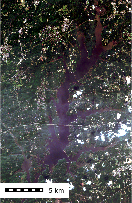

Temporal Map Calculations

Run a temporal map calculation on your entire STRDS to generate an NDVI layer.

gs.run_command(
    "t.rast.mapcalc",
    inputs=["sentinel_2.nir", "sentinel_2.red"],
    output="ndvi",
    basename="ndvi",
    method="follows",
    expression=(
        "float(if('sentinel_2.nir' >= 10000, 10000, 'sentinel_2.nir') - if('sentinel_2.red' >= 10000, 10000, 'sentinel_2.red')) / (if('sentinel_2.nir' >= 10000, 10000, 'sentinel_2.nir') + if('sentinel_2.red' >= 10000, 10000, 'sentinel_2.red'))"
    ),
    overwrite=True,
    flags="n",
)

Check to see it worked.

gs.run_command("t.list", type="strds")

ndvi@PERMANENT
sentinel_2@PERMANENT

and plot the NDVI

strds_df = pd.DataFrame(
    gs.parse_command(
        "t.rast.list",
        input="ndvi",
        order="start_time",
        columns=["name", "semantic_label", "start_time", "end_time", "min", "max"],
        format="csv",
    )
)

# Convert start_time to datetime for better formatting
strds_df["start_time"] = pd.to_datetime(strds_df["start_time"])

sns.lineplot(
    x="start_time", y="max", data=strds_df
)

# Format x-axis labels for better readability
import matplotlib.dates as mdates
import matplotlib.pyplot as plt

plt.gca().xaxis.set_major_formatter(mdates.DateFormatter('%Y-%m-%d'))
plt.gcf().autofmt_xdate()  # Auto-rotate date labels
plt.show()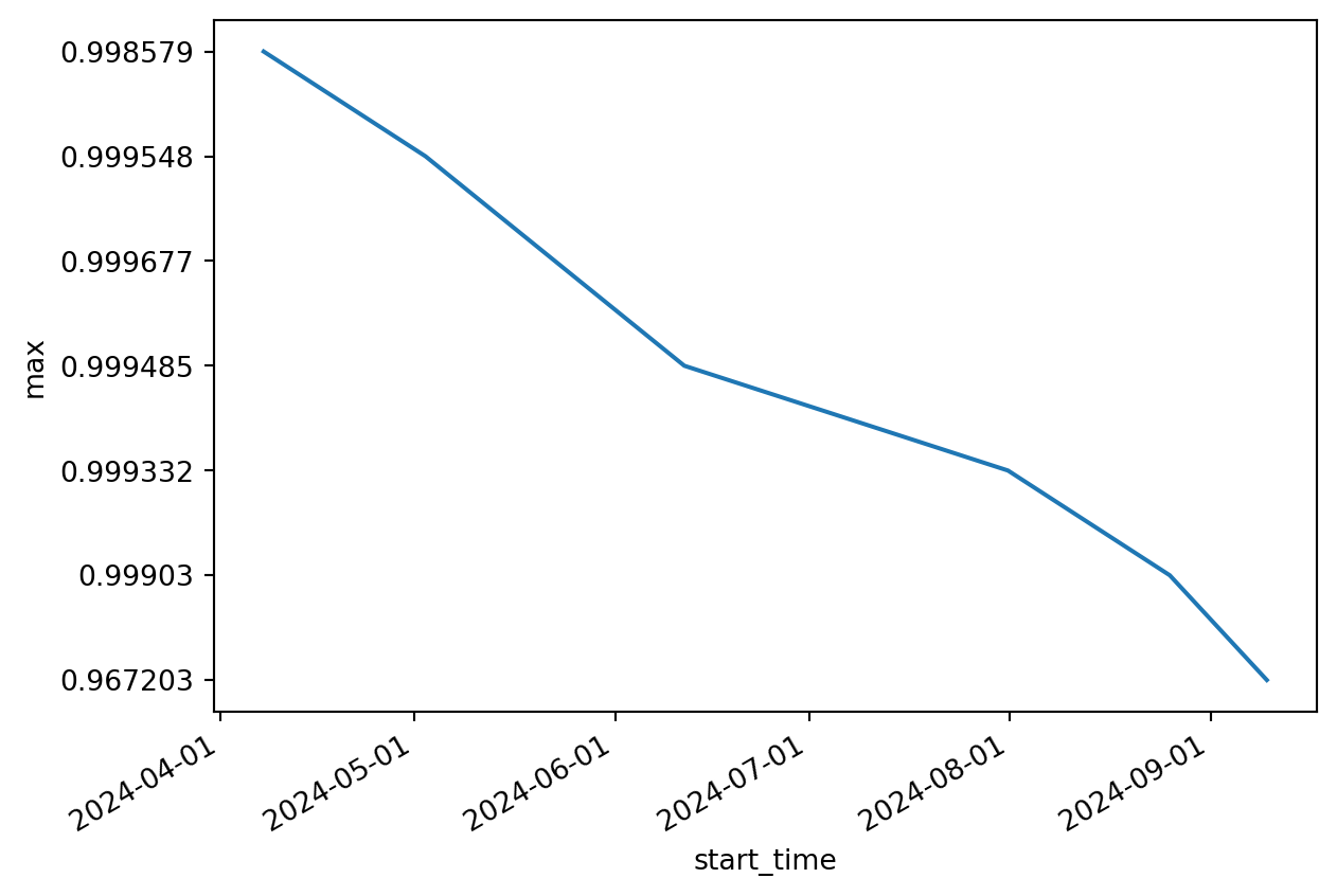

ndvi_list = gs.parse_command(
    "t.rast.list",
    input="ndvi",
    order="start_time",
    columns=["name", "semantic_label", "start_time", "end_time", "min", "max"],
    format="csv",
)
gs.run_command("t.rast.colors", input="ndvi", color="ndvi")

for ndvi in ndvi_list:
    map_name = ndvi.get("name")
    m = gj.Map(use_region=True, width=500)
    m.d_rast(map=map_name)
    m.d_barscale()
    m.d_legend(raster=map_name, flags="b")
    m.show()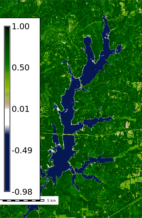

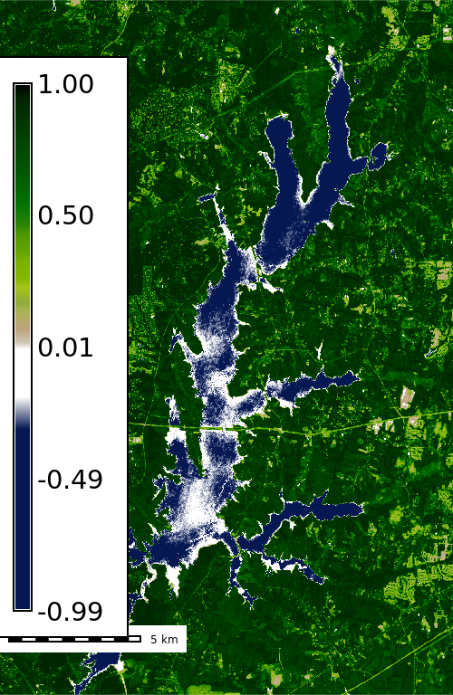
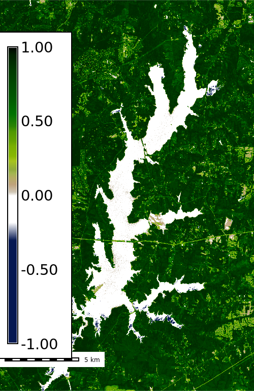
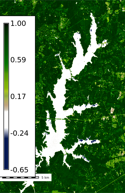
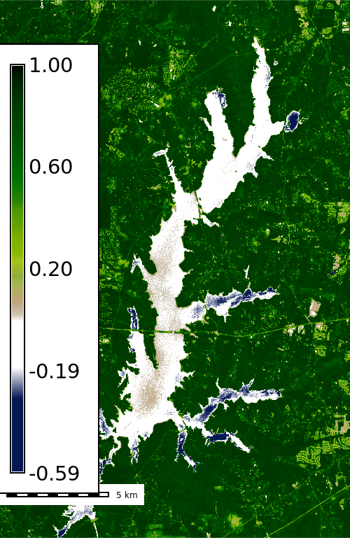
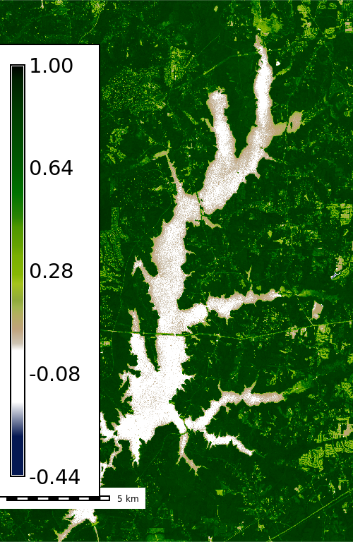
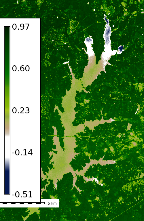
Use the series map to view the entire time series of NDVI maps in one interactive map or save as a GIF.

ndvi_rasters = [
    i.get("name")
    for i in gs.parse_command(
        "t.rast.list",
        input="ndvi",
        order="start_time",
        columns=["name"],
        format="csv",
    )
]

# Create Time Series Map
m = gj.SeriesMap(use_region=True, width=500)
m.add_rasters(rasters=ndvi_rasters)
m.d_barscale()
m.render()
m.save("outputs/ndvi_time_series.gif")

'outputs/ndvi_time_series.gif'