Satellite archives are full of before-and-after stories, but a static pair of images rarely does them justice. A well-made animation does: it lets the eye follow where and how the change happened. This post introduces r.anim.morph, a new GRASS addon that builds smooth, spatially-aware transitions between two rasters, and pairs it with t.stac to pull the imagery straight from a SpatioTemporal Asset Catalog.
Our subject is Falls Lake, the managed reservoir north of Raleigh, North Carolina. We will take a full year of Sentinel-2 passes, from 25 July 2025 to today, find two cloud-free scenes that bracket the window, and animate the reservoir’s shoreline as the 2025 to 2026 drought draws it down.
r.anim.morph contraction plan applied to Sentinel-2 true-color bands. As the water recedes, a bright fringe of exposed lakebed emerges along every cove. (Download the MP4.)
Why animate at all?
The insight behind the Baia framework (Lobo, Appert and Pietriga, 2019) is that a convincing before-and-after animation requires different pixels to transition at different times. A naive cross-dissolve fades the whole frame uniformly and reads as a blur. To make a shrinking lake look like it is actually shrinking, the pixels far from the final shoreline should disappear first and the pixels near the final shoreline should disappear last. That ordering is what r.anim.morph computes.
Given a before raster, an after raster, and a description of the change, r.anim.morph produces an animation plan: two rasters, S and E, that store for every pixel the normalized time its transition starts and ends. Each output frame at time t is then a per-pixel blend:
\[ \alpha(i,j,t) = \mathrm{clamp}\!\left(\frac{t - S_{ij}}{E_{ij} - S_{ij}},\, 0,\, 1\right), \qquad \mathrm{frame}(i,j,t) = (1-\alpha)\,\mathrm{before}_{ij} + \alpha\,\mathrm{after}_{ij} \]
r.anim.morph ships a family of primitives that generate the plan for you: blend, appearance, disappearance, contraction, expansion, deformation, radial, directional, and dem. A receding reservoir is the textbook case for contraction.
Both tools are GRASS addons installable with g.extension:
- t.stac searches and imports STAC assets (here, Sentinel-2 L2A from Earth Search).
- r.anim.morph builds the animation plan and renders the frames.
Everything else (r.mapcalc, r.import, g.region, d.rgb) is core GRASS.
Every step is shown twice: as terminal commands and as Python through the grass.tools API (GRASS 8.5 or newer). Pick a tab once and the whole post follows.
1. Set up a project and install the addons
Falls Lake sits in North Carolina, so we work in the state plane projection EPSG:3358 (NAD83 / North Carolina, meters). Create a project, then install the two addons. In Python the project is opened once with grass.script.setup and every later snippet reuses the same tools object.
import os

import grass.script as gs
from grass.tools import Tools

# One-time: create a project in NC State Plane meters
project = os.path.expanduser("~/grassdata/falls_lake")
gs.create_project(project, epsg="3358")

# Open the project; the session stays open for the rest of the post
session = gs.setup.init(project)
tools = Tools(session=session)

# Install the addons into this GRASS installation
tools.g_extension(extension="t.stac")
tools.g_extension(extension="r.anim.morph")
# One-time: create a project in NC State Plane meters
grass -c EPSG:3358 ~/grassdata/falls_lake
# Install the addons into this GRASS installation
g.extension extension=t.stac
g.extension extension=r.anim.morphSet the computational region over the reservoir at Sentinel-2’s native 10 m resolution. These bounds are in EPSG:3358 and enclose the upper reach of the lake; adjust them to your own area of interest.
tools.g_region(n=268570, s=238520, e=639300, w=627590, res=10, flags="p")g.region n=268570 s=238520 e=639300 w=627590 res=10 -p2. Explore the catalog with t.stac
t.stac mirrors the STAC hierarchy: a catalog holds collections, and a collection holds items (individual acquisitions). Start at the catalog and drill down. We use the public Earth Search endpoint, which serves Sentinel-2 L2A as cloud-optimized GeoTIFFs, no credentials required.
url = "https://earth-search.aws.element84.com/v1/"

# List collections in the catalog
print(tools.t_stac_catalog(url=url).text)

# Inspect the Sentinel-2 L2A collection (extent, assets, date range)
print(tools.t_stac_collection(url=url, collection_id="sentinel-2-l2a").text)
# List collections in the catalog
t.stac.catalog url="https://earth-search.aws.element84.com/v1/"
# Inspect the Sentinel-2 L2A collection (extent, assets, date range)
t.stac.collection \
url="https://earth-search.aws.element84.com/v1/" \
collection_id="sentinel-2-l2a"Before importing anything, search the collection over our region and window and keep only near-clear scenes. The query option accepts the STAC query extension, so we filter on eo:cloud_cover.
import json

# How many low-cloud Sentinel-2 scenes intersect the region this year?
items = tools.t_stac_item(
    url=url,
    collection_id="sentinel-2-l2a",
    datetime="2025-07-25/2026-07-17",
    query=json.dumps({"eo:cloud_cover": {"lt": 10}}),
    format="json",
).json
for item in items:
    props = item["properties"]
    print(item["id"], props["datetime"][:10], props["eo:cloud_cover"])
# How many low-cloud Sentinel-2 scenes intersect the region this year?
t.stac.item \
url="https://earth-search.aws.element84.com/v1/" \
collection_id="sentinel-2-l2a" \
datetime="2025-07-25/2026-07-17" \
query='{"eo:cloud_cover":{"lt":10}}'Over the window that search returns dozens of candidate passes. For the endpoints we pick two nearly cloud-free scenes from the same Sentinel-2 tile (17SPV) so their pixels line up: S2A_17SPV_20250725_0_L2A (25 July 2025, 2.3% cloud) and S2B_17SPV_20260703_0_L2A (3 July 2026, 0.8% cloud, the last clear pass before today).
3. Import the bands you need
Add the -d flag to download and import assets. We only need four 10 m bands: green and near-infrared for water detection, plus red and blue to complete the true-color composite. The extent=region and resolution=value options clip and resample each asset to the current region as it lands, and method=bilinear reprojects from Sentinel-2’s UTM grid into our state plane project.
# Before: 25 July 2025, after: 3 July 2026
for item_id in ("S2A_17SPV_20250725_0_L2A", "S2B_17SPV_20260703_0_L2A"):
    tools.t_stac_item(
        flags="d",
        url=url,
        collection_id="sentinel-2-l2a",
        ids=item_id,
        asset_keys="green,nir,red,blue",
        method="bilinear",
        extent="region",
        resolution="value",
        resolution_value=10,
        memory=1000,
        nprocs=4,
    )
# Before: 25 July 2025
t.stac.item -d \
url="https://earth-search.aws.element84.com/v1/" \
collection_id="sentinel-2-l2a" \
ids="S2A_17SPV_20250725_0_L2A" \
asset_keys="green,nir,red,blue" \
method=bilinear extent=region \
resolution=value resolution_value=10 \
memory=1000 nprocs=4
# After: 3 July 2026
t.stac.item -d \
url="https://earth-search.aws.element84.com/v1/" \
collection_id="sentinel-2-l2a" \
ids="S2B_17SPV_20260703_0_L2A" \
asset_keys="green,nir,red,blue" \
method=bilinear extent=region \
resolution=value resolution_value=10 \
memory=1000 nprocs=4t.stac names each imported raster <collection>.<item_id>.<asset>, for example sentinel-2-l2a.S2A_17SPV_20250725_0_L2A.green. Those names are precise but awkward in r.mapcalc, so rename them to something short:
for band in ("green", "nir", "red", "blue"):
    tools.g_rename(
        raster=f"sentinel-2-l2a.S2A_17SPV_20250725_0_L2A.{band},before_{band}"
    )
    tools.g_rename(
        raster=f"sentinel-2-l2a.S2B_17SPV_20260703_0_L2A.{band},after_{band}"
    )
for band in green nir red blue; do
g.rename raster="sentinel-2-l2a.S2A_17SPV_20250725_0_L2A.${band},before_${band}"
g.rename raster="sentinel-2-l2a.S2B_17SPV_20260703_0_L2A.${band},after_${band}"
doneSentinel-2 tile 17SPV sits at the edge of two orbit swaths, so different dates image different diagonal slices of the region. If you compare water area over the full region, a change in coverage masquerades as a change in water. Always restrict the comparison to the pixels both scenes actually observed:
# 1 where every band of both dates has valid data, null elsewhere
tools.r_mapcalc(
    expression="common = if(before_green > 0 && before_nir > 0"
    " && after_green > 0 && after_nir > 0, 1, null())"
)
# 1 where every band of both dates has valid data, null elsewhere
r.mapcalc expression="common = if(before_green>0 && before_nir>0 && \
after_green>0 && after_nir>0, 1, null())"Every measurement below is confined to this common footprint.
4. Delineate water with NDWI
The Normalized Difference Water Index (McFeeters, 1996) separates open water from land using the green and near-infrared bands. Water is bright in green and dark in NIR, so open water has a positive NDWI.
for t in ("before", "after"):
    tools.r_mapcalc(
        expression=f"ndwi_{t} = float({t}_green - {t}_nir)"
        f" / float({t}_green + {t}_nir)"
    )
    tools.r_mapcalc(
        expression=f"water_{t} = if(!isnull(common) && ndwi_{t} > 0.0, 1, 0)"
    )
for T in before after; do
r.mapcalc expression="ndwi_${T} = float(${T}_green - ${T}_nir) / \
float(${T}_green + ${T}_nir)"
r.mapcalc expression="water_${T} = if(!isnull(common) && \
ndwi_${T} > 0.0, 1, 0)"
doneProcessing baseline 04.00 shifted Sentinel-2 L2A reflectance by a -0.1 additive offset (a -1000 shift in raw DN). Because NDWI is a normalized ratio, computing it directly on the digital numbers lets the common scale factor cancel and keeps the denominator non-negative, which avoids the singularities you hit if you convert dark water to reflectance first. For land-cover mapping, apply the scale and offset; for a water index, DN works cleanly.
With the two masks in hand, the change is a single map algebra expression: water present on both dates is stable, water that became land is receded, and land that became water is gained.
tools.r_mapcalc(
    expression="change = if(water_before == 1 && water_after == 1, 1,"
    " if(water_before == 1 && water_after == 0, 2,"
    " if(water_before == 0 && water_after == 1, 3, null())))"
)
print(tools.r_report(map="change", units="k,p").text)
r.mapcalc expression="change = if(water_before==1 && water_after==1, 1, \
if(water_before==1 && water_after==0, 2, \
if(water_before==0 && water_after==1, 3, null())))"
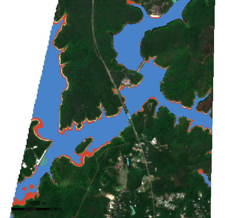
r.report map=change units=k,pOver the animated arms, the numbers tell a clear story: 3.72 km² of water on 25 July 2025 fell to 3.37 km² by 3 July 2026, a 9.4% loss. Of that, 0.39 km² of former lake became exposed shoreline while only 0.04 km² was newly flooded.
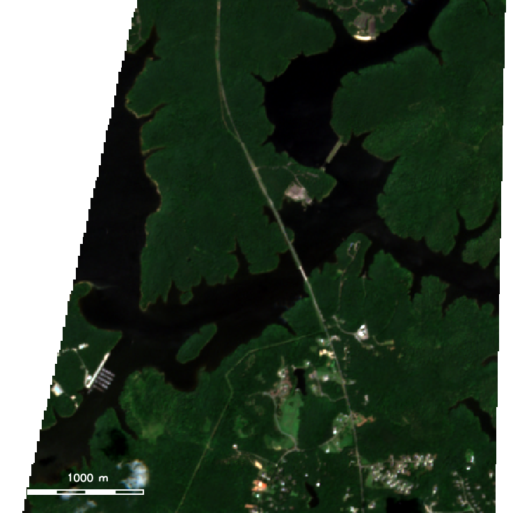
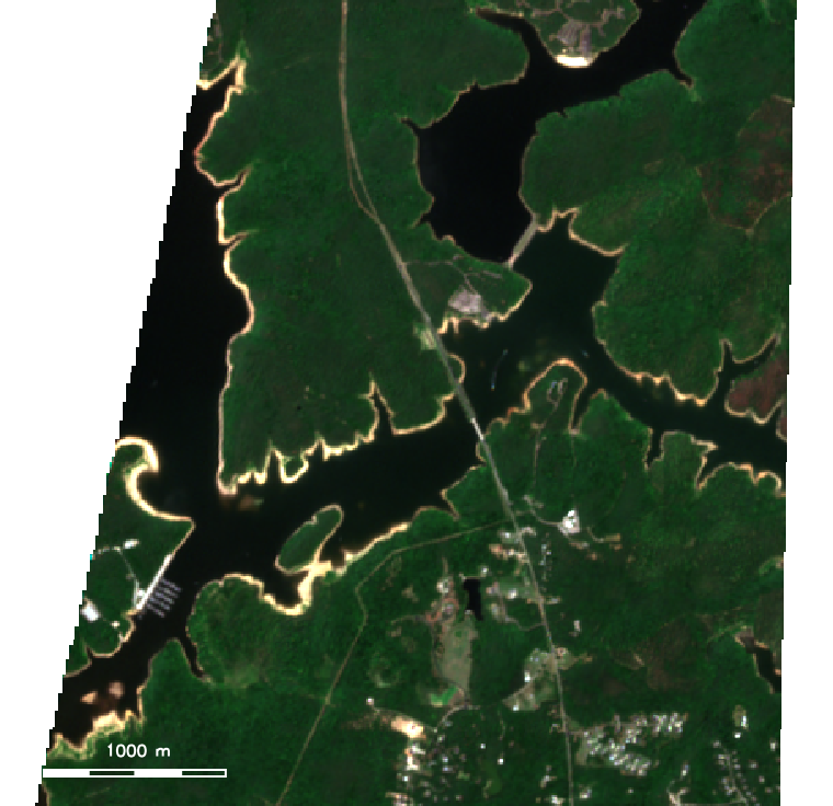
The before-and-after true-color composites show the same thing directly: the after image grows a bright tan rim of freshly exposed sediment around every finger of the lake.
5. Build the animation with r.anim.morph
Now the payoff. We hand r.anim.morph the true-color bands for each date and the two water masks, and ask for a contraction primitive. First zoom the region to the upper Cheek Creek and Ledge Creek arms, where the drawdown is easiest to see; every frame and figure below uses this window. Because the animation runs over the pixel values directly, then stretch each band to a 0 to 255 display range with a common min and max, and clip it to the common footprint. The same stretch is applied to both dates so their colors are comparable:
tools.g_region(n=253700, s=249290, e=639420, w=634870, res=10, flags="p")


# 1-99 percentile stretch per band: red 157-2333, green 218-2236, blue 198-2064
def stretch(src, lo, hi, dst):
    tools.r_mapcalc(
        expression=f"{dst} = if(isnull(common), null(),"
        f" round(255.0 * (min(max({src}, {lo}), {hi}) - {lo}) / ({hi} - {lo})))"
    )


bounds = {"red": (157, 2333), "green": (218, 2236), "blue": (198, 2064)}
for band, (lo, hi) in bounds.items():
    stretch(f"before_{band}", lo, hi, f"bef_{band}8")
    stretch(f"after_{band}", lo, hi, f"aft_{band}8")
g.region n=253700 s=249290 e=639420 w=634870 res=10 -p
# 1-99 percentile stretch per band: red 157-2333, green 218-2236, blue 198-2064
stretch() { # stretch <src> <lo> <hi> <dst>
r.mapcalc expression="$4 = if(isnull(common), null(), \
round(255.0 * (min(max($1, $2), $3) - $2) / ($3 - $2)))"
}
stretch before_red 157 2333 bef_red8
stretch before_green 218 2236 bef_green8
stretch before_blue 198 2064 bef_blue8
stretch after_red 157 2333 aft_red8
stretch after_green 218 2236 aft_green8
stretch after_blue 198 2064 aft_blue8With bef_red8, bef_green8, bef_blue8 and their aft_ counterparts in hand, build the animation:
tools.r_anim_morph(
    before="bef_red8,bef_green8,bef_blue8",
    after="aft_red8,aft_green8,aft_blue8",
    output="fl",
    primitive="contraction",
    mask_before="water_before",
    mask_after="water_after",
    roi_start=0.0,
    roi_end=0.85,
    bg_start=0.85,
    bg_end=1.0,
    blend_duration=0.25,
    frames=48,
    output_plan="fl_plan",
)

# Read the plan statistics back as JSON and list the frames
plan = tools.r_univar(map="fl_plan_S", format="json")
print(f"start times run from {plan['min']:.2f} to {plan['max']:.2f}")
frames = tools.g_list(type="raster", pattern="fl_b1_*").text.split()
print(f"{len(frames)} frames per band")
r.anim.morph \
before=bef_red8,bef_green8,bef_blue8 \
after=aft_red8,aft_green8,aft_blue8 \
output=fl \
primitive=contraction \
mask_before=water_before \
mask_after=water_after \
roi_start=0.0 roi_end=0.85 \
bg_start=0.85 bg_end=1.0 \
blend_duration=0.25 \
frames=48 \
output_plan=fl_planA few options are worth calling out:
primitive=contractionreads both masks and orders the transition so the water farthest from the new shoreline recedes first. This is what makes the lake look like it is draining rather than dissolving.- Staging (
roi_start/roi_endversusbg_start/bg_end) lets the water animate over the first 85% of the timeline while the surrounding land settles at the very end, keeping attention on the shoreline. output_plan=fl_plansaves the computedSandErasters so you can inspect or reuse the plan.- In Python, flags go in a string (
flags="c"matches the before bands to the after bands) andoverwrite=Truereplaces existing frames.
That saved plan is the clearest window into how the framework thinks. Mapping fl_plan_S, the per-pixel start time, shows the spatial ordering the contraction primitive built: the shoreline fringe (low start times) begins transitioning immediately, while the stable core and the background hold until later.
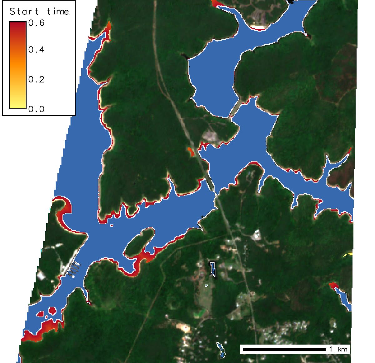
r.anim.morph writes one raster per band per frame, named fl_b1_01, fl_b2_01, fl_b3_01, and so on through frame 48. You can play them inside GRASS with g.gui.animation, or compose the three bands of each frame into RGB and export a video.
6. Export to GIF and MP4
Render each frame’s three bands to a true-color PNG, then let ffmpeg (or ImageMagick convert) assemble them. The display drivers read their settings from GRASS_RENDER_* environment variables, so in Python they go into the env of a second Tools object.
import subprocess

# Composite each frame to a PNG with the cairo driver
env = os.environ.copy()
env.update(
    GRASS_RENDER_IMMEDIATE="cairo",
    GRASS_RENDER_FILE_READ="TRUE",
    GRASS_RENDER_WIDTH="760",
    GRASS_RENDER_HEIGHT="736",
)
render = Tools(env=env)
for f in range(1, 49):
    label = f"{f:02d}"
    for b in (1, 2, 3):
        render.r_colors(map=f"fl_b{b}_{label}", color="grey255")
    env["GRASS_RENDER_FILE"] = f"frame_{label}.png"
    render.d_erase()
    render.d_rgb(red=f"fl_b1_{label}", green=f"fl_b2_{label}", blue=f"fl_b3_{label}")

# Assemble a looping MP4
subprocess.run(
    ["ffmpeg", "-framerate", "15", "-i", "frame_%02d.png", "-c:v", "libx264",
     "-pix_fmt", "yuv420p", "-crf", "20", "falls_lake_anim_morph.mp4"],
    check=True,
)
# Composite each frame to a PNG with the cairo driver
export GRASS_RENDER_IMMEDIATE=cairo GRASS_RENDER_FILE_READ=TRUE
export GRASS_RENDER_WIDTH=760 GRASS_RENDER_HEIGHT=736
for f in $(seq -w 1 48); do
for b in 1 2 3; do r.colors map=fl_b${b}_${f} color=grey255; done
export GRASS_RENDER_FILE="frame_${f}.png"
d.erase
d.rgb red=fl_b1_${f} green=fl_b2_${f} blue=fl_b3_${f}
done
# Assemble a looping MP4 and a high-quality GIF
ffmpeg -framerate 15 -i frame_%02d.png -c:v libx264 \
-pix_fmt yuv420p -crf 20 falls_lake_anim_morph.mp4
ffmpeg -framerate 15 -i frame_%02d.png -vf \
"scale=620:-1:flags=lanczos,palettegen" palette.png
ffmpeg -framerate 15 -i frame_%02d.png -i palette.png \
-lavfi "scale=620:-1:flags=lanczos[x];[x][1:v]paletteuse" \
falls_lake_anim_morph.gifThe result is the animation at the top of this post.
7. The whole reservoir
The upper arms are where the drawdown is easiest to read, but a fair question is what the whole reservoir did. Answering it exposes the footprint problem from a different angle: neither scene above covers the whole lake. Tile 17SPV is imaged from two orbits. Passes from one orbit cover the full tile; passes from the other cover only a diagonal strip, and the strip is what S2A_17SPV_20250725 and S2B_17SPV_20260703 are. The catalog tells you which is which: the s2:nodata_pixel_percentage property is 0 for a full tile and about 88 for a strip. Filter on it and two full-tile, near cloud-free passes bracket the same window: S2C_17SPV_20250726_0_L2A (26 July 2025, 0.3% cloud) and S2C_17SPV_20260701_0_L2A (1 July 2026, 0.7% cloud), both from Sentinel-2C on the full-coverage orbit.
Import them over a region that encloses the whole reservoir and rerun the same steps: common footprint, NDWI masks, stretch, r.anim.morph. Only the names, the region, and the stretch bounds change, so the code is condensed.
from io import StringIO

tools.g_region(n=264000, s=238520, e=652030, w=627590, res=10, flags="p")
scenes = (("S2C_17SPV_20250726_0_L2A", "lb"), ("S2C_17SPV_20260701_0_L2A", "la"))
for item_id, prefix in scenes:
    tools.t_stac_item(
        flags="d", url=url, collection_id="sentinel-2-l2a", ids=item_id,
        asset_keys="green,nir,red,blue", method="bilinear", extent="region",
        resolution="value", resolution_value=10, memory=2000, nprocs=4,
    )
    for band in ("green", "nir", "red", "blue"):
        tools.g_rename(raster=f"sentinel-2-l2a.{item_id}.{band},{prefix}_{band}")

tools.r_mapcalc(
    expression="lcommon = if(lb_green > 0 && lb_nir > 0"
    " && la_green > 0 && la_nir > 0, 1, null())"
)
for t in ("lb", "la"):
    tools.r_mapcalc(
        expression=f"ndwi_{t} = float({t}_green - {t}_nir) / float({t}_green + {t}_nir)"
    )
    tools.r_mapcalc(
        expression=f"water_{t} = if(!isnull(lcommon) && ndwi_{t} > 0.0, 1, 0)"
    )

# Zoom to the lake itself: clump the water of either date, keep bodies of
# 20 ha or more (ponds and cloud shadow drop out), and add a 300 m margin
tools.r_mapcalc(expression="lwater_any = if(water_lb == 1 || water_la == 1, 1, null())")
tools.r_clump(input="lwater_any", output="lwater_clumps", flags="d")
sizes = (line.split() for line in tools.r_stats(input="lwater_clumps", flags="cn").text.splitlines())
rules = "\n".join(f"{cat} = 1" for cat, cells in sizes if int(cells) >= 2000)
tools.r_reclass(input="lwater_clumps", output="lake_body", rules=StringIO(rules))
tools.g_region(zoom="lake_body", res=10)
reg = tools.g_region(flags="p", format="json")
tools.g_region(n=reg["north"] + 300, s=reg["south"] - 300,
               e=reg["east"] + 300, w=reg["west"] - 300)
reg = tools.g_region(flags="p", format="json")

# 1-99 percentile stretch per band: red 86-3014, green 154-3063, blue 95-3070
bounds = {"red": (86, 3014), "green": (154, 3063), "blue": (95, 3070)}
for band, (lo, hi) in bounds.items():
    for t in ("lb", "la"):
        tools.r_mapcalc(
            expression=f"{t}_{band}8 = if(isnull(lcommon), null(),"
            f" round(255.0 * (min(max({t}_{band}, {lo}), {hi}) - {lo}) / ({hi} - {lo})))"
        )

tools.r_anim_morph(
    before="lb_red8,lb_green8,lb_blue8",
    after="la_red8,la_green8,la_blue8",
    output="lake",
    primitive="contraction",
    mask_before="water_lb",
    mask_after="water_la",
    roi_start=0.0,
    roi_end=0.85,
    bg_start=0.85,
    bg_end=1.0,
    blend_duration=0.25,
    frames=48,
    output_plan="lake_plan",
)

# Render at the region's own size so every cell keeps its 10 m footprint,
# then let ffmpeg scale the video down
env = os.environ.copy()
env.update(
    GRASS_RENDER_IMMEDIATE="cairo",
    GRASS_RENDER_FILE_READ="TRUE",
    GRASS_RENDER_WIDTH=str(reg["cols"]),
    GRASS_RENDER_HEIGHT=str(reg["rows"]),
)
render = Tools(env=env)
for f in range(1, 49):
    label = f"{f:02d}"
    for b in (1, 2, 3):
        render.r_colors(map=f"lake_b{b}_{label}", color="grey255")
    env["GRASS_RENDER_FILE"] = f"lake_{label}.png"
    render.d_erase()
    render.d_rgb(red=f"lake_b1_{label}", green=f"lake_b2_{label}", blue=f"lake_b3_{label}")
subprocess.run(
    ["ffmpeg", "-framerate", "15", "-i", "lake_%02d.png",
     "-vf", "scale=-2:1000:flags=lanczos", "-c:v", "libx264",
     "-pix_fmt", "yuv420p", "-crf", "25", "falls_lake_whole_anim_morph.mp4"],
    check=True,
)
g.region n=264000 s=238520 e=652030 w=627590 res=10 -p
for item in S2C_17SPV_20250726_0_L2A S2C_17SPV_20260701_0_L2A; do
t.stac.item -d \
url="https://earth-search.aws.element84.com/v1/" \
collection_id="sentinel-2-l2a" ids="$item" \
asset_keys="green,nir,red,blue" \
method=bilinear extent=region \
resolution=value resolution_value=10 \
memory=2000 nprocs=4
done
for band in green nir red blue; do
g.rename raster="sentinel-2-l2a.S2C_17SPV_20250726_0_L2A.${band},lb_${band}"
g.rename raster="sentinel-2-l2a.S2C_17SPV_20260701_0_L2A.${band},la_${band}"
done
r.mapcalc expression="lcommon = if(lb_green>0 && lb_nir>0 && \
la_green>0 && la_nir>0, 1, null())"
for T in lb la; do
r.mapcalc expression="ndwi_${T} = float(${T}_green - ${T}_nir) / \
float(${T}_green + ${T}_nir)"
r.mapcalc expression="water_${T} = if(!isnull(lcommon) && \
ndwi_${T} > 0.0, 1, 0)"
done
# Zoom to the lake itself: clump the water of either date, keep bodies of
# 20 ha or more (ponds and cloud shadow drop out), and add a 300 m margin
r.mapcalc expression="lwater_any = if(water_lb==1 || water_la==1, 1, null())"
r.clump -d input=lwater_any output=lwater_clumps
r.stats -cn input=lwater_clumps | awk '$2 >= 2000 {print $1 " = 1"}' \
| r.reclass input=lwater_clumps output=lake_body rules=-
g.region zoom=lake_body res=10
eval $(g.region -g)
g.region n=$((n+300)) s=$((s-300)) e=$((e+300)) w=$((w-300)) -p
# 1-99 percentile stretch per band: red 78-3370, green 144-3349, blue 90-3337
stretch() { # stretch <src> <lo> <hi> <dst>, clipped to lcommon
r.mapcalc expression="$4 = if(isnull(lcommon), null(), \
round(255.0 * (min(max($1, $2), $3) - $2) / ($3 - $2)))"
}
for T in lb la; do
stretch ${T}_red 86 3014 ${T}_red8
stretch ${T}_green 154 3063 ${T}_green8
stretch ${T}_blue 95 3070 ${T}_blue8
done
r.anim.morph \
before=lb_red8,lb_green8,lb_blue8 \
after=la_red8,la_green8,la_blue8 \
output=lake \
primitive=contraction \
mask_before=water_lb \
mask_after=water_la \
roi_start=0.0 roi_end=0.85 \
bg_start=0.85 bg_end=1.0 \
blend_duration=0.25 \
frames=48 \
output_plan=lake_plan
# Render at the region's own size so every cell keeps its 10 m footprint,
# then let ffmpeg scale the video down
eval $(g.region -g)
export GRASS_RENDER_IMMEDIATE=cairo GRASS_RENDER_FILE_READ=TRUE
export GRASS_RENDER_WIDTH=$cols GRASS_RENDER_HEIGHT=$rows
for f in $(seq -w 1 48); do
for b in 1 2 3; do r.colors map=lake_b${b}_${f} color=grey255; done
export GRASS_RENDER_FILE="lake_${f}.png"
d.erase
d.rgb red=lake_b1_${f} green=lake_b2_${f} blue=lake_b3_${f}
done
ffmpeg -framerate 15 -i lake_%02d.png -vf "scale=-2:1000:flags=lanczos" \
-c:v libx264 -pix_fmt yuv420p -crf 25 falls_lake_whole_anim_morph.mp4Over the whole reservoir the change is no longer subtle. 29.0 km² of water on 26 July 2025 became 18.8 km² on 1 July 2026, a 35% loss: 10.8 km² of former lake surface was exposed while 0.7 km² was newly counted as water. The main body near the dam stays wet and forms the stable core of the plan; the shallow upper reaches at the northwest end of the lake drain almost entirely, which is why they animate first and longest. Two artifacts of the scenes are worth knowing. The water surface reads bright grey in the 1 July 2026 pass, most likely sun glint from that orbit’s view angle, so the main body brightens even where it stays wet. And most of the newly counted water is cloud shadow, which NDWI reads as water; masking with the scene classification asset would remove it, and the same scattered cumulus is visible in the frames.
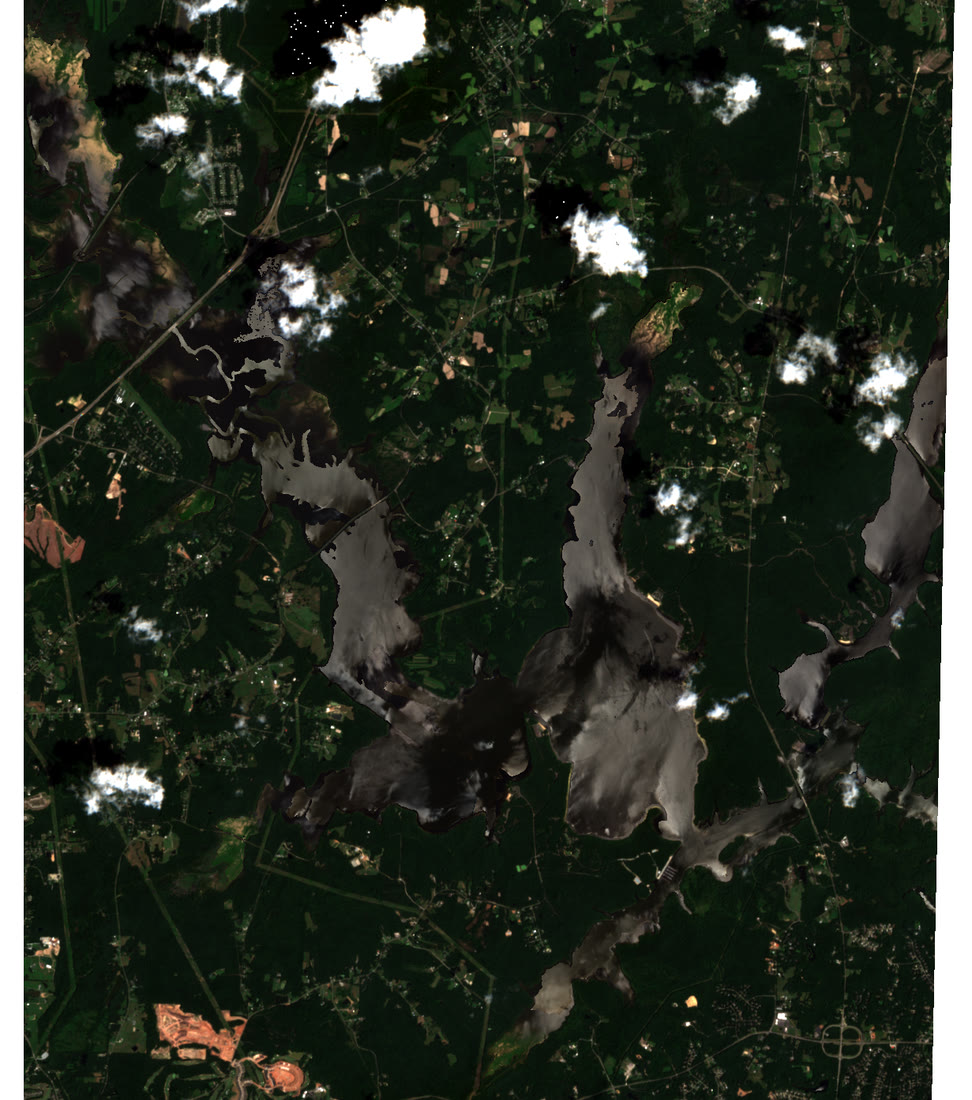
The drought behind the animation
The two dates bracket the 2025 to 2026 drought. Falls Lake is a US Army Corps of Engineers reservoir with a normal pool of 251.5 feet, and the 25 July 2025 scene shows it close to that level, just before a dry fall opened the driest year North Carolina has recorded since 1895. Raleigh Water entered Stage 1 restrictions on 20 April 2026 when water-supply storage fell to 85%. By mid June the lake was 5.3 feet below normal pool at 66% storage, Wake County was in extreme drought, and most of Durham County was in exceptional drought, the highest category on the U.S. Drought Monitor. On 9 July the USGS gauge read 245.27 feet, about six feet below normal, the lowest the lake had been since the 2007 to 2008 drought, and the Corps had it on pace for its driest June on record. The 3 July scene sits within days of that low point. Rain in late July lifted the lake back to 84% storage and the restrictions were lifted on 3 August, but the state’s 4 September drought update still had Falls Lake more than three feet below normal.
Set against that, the 9.4% surface-area loss over the mapped arms is only a window on it. Across the reservoir the same method finds a 35% loss of water surface (section 7), in line with the roughly one-third drop in storage the Corps reported. The arms window happens to be dominated by the deep channel that stays wet, while the shallow upper reaches of the lake lose nearly all of their surface. What area captures well in either case is where the change happened: gently shelving shorelines expose a wide, continuous band of lakebed along every cove, and that is what r.anim.morph turns into something you can watch. Sources: WRAL reporting from 16 June and 8 July 2026, the N.C. Drought Management Advisory Council, and the Corps’ Falls Lake water management data.
That is the real value of pairing the two tools. t.stac makes a year of analysis-ready Sentinel-2 a couple of commands away, and r.anim.morph turns a pair of dates into a spatially-honest animation whose motion shows where the change happened. Swap the primitive to expansion for a flood, dem for snow accumulating down from the peaks, or directional for a fire front, and the same workflow retells a very different story.
Reproduce this
- r.anim.morph manual and source: OSGeo/grass-addons
- t.stac manual: grass.osgeo.org
- GRASS downloads and documentation: grass.osgeo.org
- Earth Search STAC endpoint: element84.com/earth-search
Sentinel-2 data are courtesy of the Copernicus programme (ESA), served as cloud-optimized GeoTIFFs by Element 84 on AWS.
Built with GRASS, the free and open-source geospatial processing engine, and published on OpenPlains Learning.